FULL RESEARCH ARTICLE

Robert M. Sullivan*

Northern California Wildlife Ecology and Fisheries Sciences, Weaverville, CA 96093, USA

*Corresponding Author: robert.m.sullivan@icloud.com; https://www.researchgate.net/profile/Robert-Sullivan-4

Published 22 November 2022 • www.doi.org/10.51492/cfwj.108.20

Abstract

I evaluated trends in spatial and temporal variability in historical levels of rainfall, water elevation, and breach events for lakes Earl, Tolowa, and their combined lagoon system along the coast of northern California. I examined the efficacy of time series analyses to model and forecast rainfall and lake elevation at a regional scale from 2008 to 2021. I employed semi-parametric Generalized Additive Model regression to investigate the historical relationship between anthropogenic breaching of the lagoon and simultaneous occurrences of environmental parameters to better understand conditions surrounding each breach event. Evaluation of the central tendency of rainfall and surface lake elevation showed high fluctuations in their mean, positive skewed, and leptokurtic curves. Augmented Dickey-Fuller tests found that seasonal rainfall was stationary, but surface lake elevation attained stationarity only after the first seasonal difference. Decomposition of each time series and MannKendall and Sen’s slope estimators, found a significant decreasing trend in seasonal surface lake elevation but no trend was found in rainfall. Seasonal Autoregressive Integrated Moving Average (SARIMA) time series analysis and diagnostic tests of stability and reliability found best fit models for rainfall (SARIMA[1,0,0] [2,1,1]12) and surface lake elevation (SARIMA [1,1,2] [1,0,0]12) used to forecast future values for each parameter. Multiple regression of variables obtained at each breach event showed that the proportion of variance (55.0%) and null deviance (72.1%) explained by the combination of rainfall, hightide, and wave height was the “best” model with the lowest Generalized Cross-Validation statistic of all other models evaluated. All models agreed that rainfall was the most significant factor within each set of predictor attributes used to model surface lake elevation. A declining trend in surface elevation in combination with variation in the historical area and extent of wetland plant communities may be attributable to systematic breaching of the lagoon annually.

Key words: anthropogenic, forecast, GAM, historical data, resource management, SARIMA, trend

Citation: Sullivan, R. M. 2022. Time series modeling of rainfall and lake elevation in relation to breaching events at the Lake Earl and Tolowa lagoon system, coastal northern California. California Fish and Wildlife Journal 108:e22.

Editor: Felipe La Luz, Fisheries Branch

Submitted: 21 February 2022; Accepted: 22 June 2022

Copyright: ©2022, Sullivan. This is an open access article and is considered public domain. Users have the right to read, download, copy, distribute, print, search, or link to the full texts of articles in this journal, crawl them for indexing, pass them as data to software, or use them for any other lawful purpose, provided the authors and the California Department of Fish and Wildlife are acknowledged.

Competing Interests: The author has not declared any competing interests.

---

Introduction

To understand recent and future climatic trends and future climatic change it is necessary to examine the nature of past variability in climate (Nicholls et al. 2012). Time series analysis is a specific way of analyzing a sequence of data points collected over a consistent interval of time (Hyndman and Athanasopoulos 2018). Use of time series modeling is an important tool in the management of environmental data and management of natural resources (i.e., weather, rainfall, temperature, flow rate, etc.; Papalaskaris et al. 2016; Papalaskaris and Kampas 2017; Dimri et al. 2020; Martínez et al. 2020; Sullivan and Hileman 2020). Historically, the prediction of such events has always been the subject of intense interest to resource managers, not only from an ecosystem perspective but also from an economic and public safety viewpoint. This is because time series modeling helps land managers identify trends, patterns, and processes that are useful in understanding the potential causes of various phenomenon over time. Not only is time series used in forecasting future events based on historical data, but the methodology is also useful in pattern recognition, benchmarking, evaluating the influence of a single factor on the time series, and in quality control (Stoffer and Shumway 2019). Variance in success of natural resource management actions across time periods can also be used to highlight a problem, the tracking of which may enable land managers to take remedial measures in relation to seasonality, trends, rare events, and anthropogenetic disruptions in specific environmental processes or events.

In coastal lagoon systems modeling to forecast rainfall and surface lake elevation is important in evaluating ecosystem processes and trends in biological diversity that have major land management implications. A significant aspect of hydrometeorology time series modeling also involves predictions about, and attempts to mitigate, the effects of increasing lake or river levels and flow preceding precautionary needs to artificially breach lagoon systems, and in evaluating and formulating administrative breaching policy. Lakes Earl and Tolowa, and their combined lagoon system, consists of a complex landscape mosaic of coastal habitat with a diverse array of flora and fauna including sensitive plant and animal species. This lagoon ecosystem was identified as one of California’s 19 most productive wetlands and has been a California Department of Fish and Wildlife (CDFW) acquisition priority since 1975. Together both lakes constitute the largest lagoon system, and the third-most important seabird area on the West Coast after the Farallon and the Channel Islands in southern California. The largely freshwater Lake Earl and somewhat brackish Lake Tolowa ecosystems comprise an important avian habitat while the surrounding area is used for habitation and recreation. These waters also provide habitat for many federal and State special status species of plants and animals. The Audubon Society has identified this region as one of the most ornithologically significant coastal bird habitation and recreation centers in the State. Lake Earl is also a significant component in the Flood Control Plan for the County of Del Norte and breaching of the lake’s sandbar is vital to the functioning of onsite wastewater systems and wells, and for management of runoff from storms and seasonal rains. 

Although the Lake Earl Wildlife Area (LEWA) management plan seeks to optimize habitat for a variety of plant and animal communities, as well as striking a balance between management of natural resources, agriculture, and private property concerns, the necessary integrated analysis of hydrological, ecological, and physical processes of the lagoon system in relation to biological communities and the marine environment has not been thoroughly quantified or modeled (Tetra Tech 2000; Anderson 2002; Anderson and Schlosstein 2003; Lowe 2003; Kraus et al. 2008). In an attempt to initiate this process my main objectives were: 1) conduct trend analysis of the long-term hydrometeorological events in the Lake Earl-Tolowa lagoon complex to determine if seasonal variance in rainfall and surface lake elevation change significantly over time; 2) determine the dependency of individual rainfall and surface lake elevation events on their preceding events to see if each time series is random stationary or nonstationary; 3) gauge the extent of cross-correlation between rainfall and surface lake elevation; 4) use SARIMA modeling to describe, evaluate, and forecast future seasonal patterns based on the historical time series record; and 5) describe the relationship between surface lake elevation in relation to events surrounding each breach event. Placing climatically-driven historical time series models and anthropogenically driven breach events into perspective provides additional insight toward the stated goal of optimal management of wetland and aquatic resources, notwithstanding the physical processes occurring within the lagoon system and the inevitable long-term effects of climate change (Sullivan 2020).

Methods

Study Area

Lakes Earl and Tolowa are located near the town of Fort Dick, ~7.5 km north of Crescent City, Del Norte County, California (latitude ~41.8° N, longitude ~124.2° W; elevation 14 m; Fig. 1). Both lakes are contained within the LEWA and Smith River Hydrologic Unit. The combined surface area of these two lakes is ~2,023 hectares with a perimeter of ~96.6 km. This portion of the Smith River Plain or Crescent City platform (~14,164 ha) consists of a relatively flat coastal terrace at the base of the Coast Range Mountains bordering the Pacific Ocean (Anderson 2002; CDFG 2003). Lake Earl has two principal lobes separated by the “Narrows” (Fig. 1). The smaller lobe, closest to the ocean and the sandbar barrier beach site is Lake Tolowa (also referenced as “Lake Talawa”) and the larger lobe is Lake Earl.

There is a salinity gradient in Lake Earl emanating from the Narrows during open estuary conditions. Waters having the least salinity occur at the north and south extremes of Lake Earl (Tetra Tech 2000). Inflow (~80%) of water into the lake and lagoon system is derived directly from precipitation onto the surface of each lake, streamflow (i.e., Jordan, Yonkers and other unnamed creeks) within the surrounding watershed, groundwater seepage (~20%) from the Smith River Plain (Anderson 2002), and some tidal inflow when the lagoon is breached (Anderson 2002; Anderson and Schlosstein 2003; Kraus et al. 2002, 2008). Outflow of water from the lagoon occurs through wet-season breaching, dry-season evaporation, and ground water seepage, which lowers the water level in the summer. Lakes Earl and Tolowa fluctuate in elevation with winter rains impounded by a sandbar barrier beach at the mouth of the lagoon in summer (Anderson 2002; Fig. 1).

Typically, the barrier beach consists of a long and narrow sand body aligned parallel to the coast that forms between the ocean and the entrance to the lagoon that is not submerged by the tide (Kraus et al. 2008). The barrier beach separating the lagoon from the Pacific Ocean breaches periodically, either naturally or mechanically, opening the lagoon to the ocean. Sand then builds back up over time and the lagoon closes. Coastal sand dune habitat extending inland from the ocean is covered with scattered European beach grass (Ammophila arenaria), sand verbena (Abronia latifolia), and a variety of other grasses and forbs. Inland areas transition through grassland and pasture habitat ending in upland Coastal maritime forests of Sitka spruce (Picea sitchensis), grand fir (Abies grandis), and beach or shore pine (Pinus contorta ssp. contorta). 

Data Collection

Historical data for total monthly rainfall (cm) and maximum monthly lake elevation (m) were collected from the National Oceanic and Atmospheric Administration (NOAA), McNamara Airport, Crescent City (lat. 41.7836°, long. -124.2380°, elev. 17 m)¹; and the California Department of Water Resources Data Exchange Center (CDEC) website for the Earl Lake Fort Dick Station (EFD; lat. 41.8428, long. -124.1886, elevation 3 m)², respectively. In addition to rainfall and lake elevation data, I also obtained several marine environmental variables for use in evaluating the circumstances surrounding each breach event, including maximum marine: 1) hightide, 2) wind direction, 3) wind speed, 4) wind gust, 5) wave height, and 6) dominant wave period at the time of each breach event. These data were collected on the day of each breach event and downloaded from the NOAA Station, Crescent City.^3,4 Dominant wave period is representative of the highest waves encountered during the sampling period. I note that complete digital datasets were lacking for all environmental attributes from each of the aforementioned sources for the years, months, or days sampled.

Breaching has occurred naturally, illegally (i.e., without permit), or mechanically under permit from the California Coastal Commission to Del Norte County and CDFW. Yet historically, the exact cause and lake elevation of many of these breach events is unknown. The date of each breach event (n = 107) ranged from 1969 forward (H. Kunstal pers. comm. 2022; K. Freeman pers. comm. 2022). Breach events accompanied by Lake Earl elevation data were available since 1987 and data on monthly maximum rainfall at the time of each breach event were available since 2000. Evaluation of historical trends in the distribution and aerial extent of major vegetation communities were assessed by use of the “baseline” vegetation map developed by Tetra Tech (2002) for the LEWA Environmental Impact Report (EIR; CDFG 2003). I clipped this baseline map at the 3.7 m contour and subsequent fluctuations in the area and location of vegetation communities were mapped onto 2010 and 2014 National Agriculture Imagery Program (NAIP) digital orthophoto quarter quad (DOQQ) photographic satellite imagery for comparisons with the 2002 baseline map (https://naip-usdaonline.hub.arcgis.com/).

Breaching

Lakes Earl and Tolowa cycle through three annual phases as a function of rainfall, watershed inflow, and breaching activity (Lowe 2003). Annual breaching generally occurs between 1 September and 15 February depending upon the water level. Follow-on breaching events also may occur in mid-February if the water surface elevation in the lakes rises above ~1.5 mean sea level (MSL). However, the actual surface elevation of Lake Earl may reach ~3.1 m MSL before breaching is completed. Mechanical breaching is designed to prevent overfilling and flooding of surrounding low-lying areas. Following a breach event water level in the lagoon tends to drop to < 1 m within two days (TetraTech 1999). From March to September the lagoon slowly refills, while losing some water through evaporation the extent to which is currently unknown for both the lake and lagoon system (Anderson 2002; Anderson and Schlosstein 2003; Kraus et al. 2008). 

According to the LEWA land management plan breaching occurs at the narrowest part of the sandbar between Lake Tolowa and Pacific Ocean. A “natural” breach of the lagoon system is a rare event. Anderson and Schlosstein (2003) estimate that if the lagoon is not manually breached, it will likely breach naturally when elevation of the lagoon reaches ~3.7 to ~4.3 m MSL. The potential for natural breaching from the lagoon side is related to the ratio formed as the water-head difference between the lagoon and ocean divided by the width of the barrier beach (Kraus et al. 2008). Historically, Native Americans occasionally breached the sand beach barrier (Lauck 1997). Currently, the lagoon system may be breached without permit by local residents or mechanically (with permit) by Del Norte County in cooperation with CDFW, approximately once a year whenever the water surface elevation of the lakes reach ~2.4 to ~3.1 m MSL. According to Lauck (1997), the philosophy behind management of surface water elevation in Lake Earl changed about 1990.

Breaching the barrier sandbar involves excavating a trench ~61-m long by ~6.0-m wide by ~2.0-m deep to start the flow of water from the lagoon system into the ocean. Once the flow is started it increases rapidly and causes additional erosion of the beach barrier sandbar (Appendix IA–IH (PDF)). After the inlet is open, tidal waters enter the lagoon freely for a few days thereafter and before the barrier sandbar reforms again due to beach dynamics. Once breaching is initiated water in the lagoon drops to the same elevation regardless of the initial surface elevation (Johnson 1976; Anderson 2002; Anderson and Schlosstein 2003; Lowe 2003). Coastal breaches of small lagoons generally close naturally by wave-driven longshore sediment transport and deposition (Smith and Zarillo 1988; Kraus et al. 2008). 

Statistical Analyses

Standard statistics.—All statistical tests used the R-suite of statistical programs (R Core Team 2022). The Anderson-Darling (AD) test statistic (Stephens 1979) showed that each environmental metric was not normally distributed (i.e., maximum monthly rain fall: AD = 2.9, P < 0.001, n = 168; maximum monthly Lake Earl elevation: AD = 6.6, P < 0.001, n = 168). I conducted a visual assessment of each environmental variable using two goodness-of-fit statistics: 1) theoretical density plots of histograms vs. fitted density functions and 2) empirical vs. theoretical quantile (Q-Q) plots with emphasis on lack-of-fit at the tails of each distribution (Delignette-Muller and Dutang 2015; Appendix IIA-IID (PDF)). Multiple goodness-of-fit-criteria showed that each environmental parameter most closely fit a theoretical Gamma distribution consistent with visual assessments of the distribution of each parameter and goodness-of-fit-statistics (Akaike’s Information Criterion [AIC], Akaike 1973; Bayesian Information Criterion [BIC]; Schwarz 1978; Burnham and Anderson 1998; Table 1). Consequently, I used non-parametric or semi-parametric statistical methods for all subsequent univariate and multivariate statistical analyses (McDonald 2014; Tsiatis et al. 2006). AIC applies to situations where there may not be “a model” but many effects of different sizes and attempts to maximize prediction error. BIC assumes the model is in the dataset being evaluated and tends to focus in on “one model” as the number of observations grow. BIC generally favors a less complex model. 

Table 1. Multiple goodness of fit criteria for the distribution of rainfall (cm) and surface lake elevation (m) from 2008 to 2021. The smaller the value for each goodness-of-fit statistic the better the fit to the theoretical frequency distribution.

Goodness-of-fit-criteria	Gamma	Normal	Weibull
Lake Earl AIC	343.0	364.0	350.0
Lake Earl BIC	350.0	371.0	357.0
Rainfall AIC	1,171.0	1,313.0	1,171.0
Rainfall BIC	1,178.0	1,319.0	1,178.0

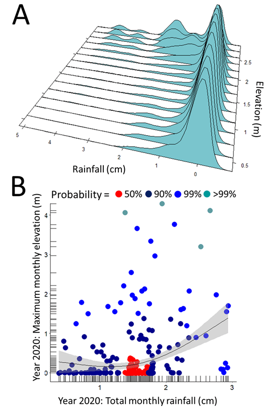
I used the gghdr program package to plot monthly boxplots of the highest density regions (HDR) of the underlying probability distribution (i.e., 50%, 90%, 99%, > 99% HDRs) in the monthly run-up to breaching illustrated for a typical year (i.e., 2020). This method summarized any multimodal distribution in the relationship between rainfall and surface lake elevation in relation to disjoint climatic (monthly) subsets for both parameters (Hyndman 1996; O’Hara-Wild et al. 2022). I used seasonal Mann-Kendall (MK, 2-tailed test; Hirsch et al. 1982; Hipel and McLeod 2005) and Sen’s slope statistics (z; Sen 1968; Hipel and McLeod 2005) to evaluate trend and significance levels in each of the historical time series (Mann 1945; Kendall 1975; Gilbert 1987). I used the Pettitt’s test (U) to identify the point at which values in the data series exhibited a change in any trend that was observed (Helsel et al. 2020). Spearman’s rank correlation statistic (r_s, 2-tailed test) calculated the strength and direction of the relationship between any two variables, expressed as a monotonic relationship, whether linear or not (Corder and Foreman 2014). Statistical significance for all tests was set at α < 0.05. 

Generalized additive model regression.—I used semiparametric Generalized Additive Modeling (GAM; Wood 2017) in all regressions of environmental variables (Hastie and Tibshirani 1990; Madsen and Thyregod 2011). A semiparametric statistical model has parametric and nonparametric components (https://en.wikipedia.org/wiki/Semiparametric_model). GAM response curves showed the relationship between the fitted function and the response variable. Smooths were “centered” to ensure model identity and summed to zero over covariate values. Statistics reported by each GAM were: 1) F-value (~significance of smooth term); 2) ~P-value and 95% confidence band for the spline line (Nychka 1988); 3) estimated (effective) degrees of freedom for the model terms (edf = P-value the test is based on); 4) adjusted regression coefficient for each model (R² adj.) defined as the proportion of the variance explained, where original variance and residual variance are both estimated using unbiased estimators; 5) proportion of null deviance explained (Dev.Exp.) taking account of any offset; and 6) the Generalized Cross-Validation criterion (GCV) or generalized error of a model, in which a score that is lower in comparison to other models represents a better fit. Ranked correlation (r_s) analysis also assessed the strength and significance of the relationship in each variable delineated by the smooth term (Diankha and Thiaw 2016). I used a Gamma error-structure (family = “Gamma” [link = “log”]) to assess fluctuations in the error distribution of each environmental variable based on results of the theoretical density and Q-Q plots.

Because of small sample size there were more coefficients than the data would allow in each GAM regression model beyond three predictors. Therefore, in evaluating attributes surrounding each breach event I retained rainfall and hightide in each multiple regression while adding each of the other variables one-by-one into the analysis. I assumed that use of rainfall and hightide as standards within each model was the most logical approach for evaluating each of the other marine parameters. In evaluating the circumstances surrounding each breach event I further assumed, as did Kraus et al. (2008), that all natural and anthropogenic breaches were initiated at the approach to maximum possible water level, or at the time of maximum lake elevation, with the intent to alleviate flooding around the lagoon perimeter.

Steps used to build SARIMA time series models.—Construction of a historical time series model may vary depending on the characteristics of the data and the research question(s). Here, I used the following basic steps in the analysis: 1) Gather historical data, plot time series, and check for outliers. 2) Determine interval of consecutive time sequence (i.e., daily, Julian week, month, year). 3) Decompose to extract trend, seasonality, and error. 4) Check if time series were stationary and evaluate correlation structure. 5) If non-stationary make stationary by differencing and check if stationary again. 6) Determine the “best fit” seasonal time series model. 7) Use diagnostics on residuals of the best fit model as a final check. 8) Run the SARIMA model with best fit parameters. 9) Forecast values into the future (~2–3 years). 10) Assess accuracy of the modeled forecast.

Stationarity, seasonal-trend decomposition and adjustment.—Continuous uninterrupted historical annual data were aggregated by month. I used the Ljung–Box test (lag = 12, type = ”Ljung-Box”) to evaluate whether data were independently distributed (i.e., no autocorrelation, when P > 0.05) and thus stationary. Parsimony was used to evaluate the performance of each model validated by use of a minimum AIC statistic. I used Seasonal-Trend decomposition using Loess (STL; Cleveland et al. 1990) in an additive model to remove the seasonal effect from each time series in an effort to understand trend-effects. In an additive model the variance of data does not change over different values in the time series. In a multiplicative model as the data increases so does the seasonal pattern or variance. The STL plot decomposition method used local polynomial regression fitted by a least squares algorithm to partition the time series of each dataset into three components: 1) trend (Tt), 2) seasonality-cycle (St), and 3) remainder (Rt), written as: yt = St + Tt + Rt, for t = 1 to N measured data points (Hydman and Khandakar 2008). The remainder (i.e., error) component equates to the residuals derived from the seasonal plus trend fit, or “random” time series (Cleveland et al. 1990, Hart1992). 

Time series modeling and seasonality.—Seasonal time series analysis assumes that successive values in the data file represent consecutive measurements taken at equally spaced time intervals (Hill and Lewicki 2007). Because all environmental data exhibited seasonality a SARIMA time series analyses was identified as an appropriate stochastic model for describing and predicting seasonal variance in rainfall and surface elevation of water in the lake-lagoon system (Machiwal and Jha 2006; Nau 2017; Shumway and Stoffer 2017; Hyndman and Athanasopoulos 2018). An Autoregressive Integrated Moving Average (ARIMA) time series is a model that uses time series data to either better understand the dataset or to predict future trends. Although ARIMA is a widely used forecasting method for univariate time series data, it does not support time series with a seasonal component. In contrast, SARIMA is an extension of the ARIMA model that is applied to an ARIMA time series that shows seasonal patterns. Elements of an ARIMA time series are written using lowercase letters, the seasonal components of the model are referenced using uppercase letters, and each fitted model is written in a specific order: SARIMA (p, d, q) (P, D, Q)S. Here, p = non-seasonal order, d = non-seasonal differencing, q = non-seasonal moving average, P = seasonal order, D = seasonal differencing, Q = seasonal moving average, and the letter S refers to the number of periods per season. The seasonal factor S = 12, indicating the time interval of consecutive monthly seasonal sequences. Differencing (d, D) was used to make a time series stationary (i.e., if not stationary) by subtracting each data point in the series from its successor (Hyndman and Athanasopoulos 2018).

Auto.arima, autocorrelation, and forecasting.—The auto.arima function with drift was used to determine the order of each time series. Here the algorithm conducts numerous iterations and checks in search of all possible models within the order of constraints provided (Hyndman and Khandakar 2008). This stepwise algorithm automatically returns the best “fit” model with the lowest AIC and BIC values (Wang et al. 2006). Each time series model was evaluated graphically by inspection of theoretical density histograms and normal Q-Q plots of residuals, and associated P-values. I used the Ljung-Box test (Q*) to check if autocorrelation existed among residuals within each time series, as it is the most important precondition for time series analysis and forecasting (Box and Jenkins 1970; Fuller 1976; Ljung and Box 1978). Once the best-fit model from auto.arima was identified it was passed to SARIMA from which the function sarima.for() was used to forecast a future 48-month time interval for both rainfall and lake surface elevation. Accuracy of forecasting for each SARIMA model was evaluated by use of the Mean Absolute Percentage Error (MAPE) measure (i.e., MAPE = (1/n) * Σ (|actual historical data – forecasted values| / |actual|) * 100). The lower the MAPE score the better fit to the applied model. For example, a MAPE value of < 10% or 11 – 20% is an excellent-to-good forecasting estimate, respectively (Lewis 1982; Moreno et al. 2013; Hyndman and Athanasopoulos 2018).

Results    

Annual and Seasonal Variation in Historical Data

Despite being highly variable, annual fluctuations in historical total monthly rainfall showed no significant relationship over time for the period 2008 to 2021 (F = 0.01, P = 0.95; Fig. 2A); however, maximum monthly surface elevation declined significantly over the same period (F = 6.2, P < 0.001; Fig. 2B). For the time period I studied the water level in the lagoon varied seasonally from ~-0.2 m to ~3.2 m with respect to MSL. Historical seasonal variation in both parameters exhibited the same basic pattern (Fig. 2C and 2D). Although the seasonal pattern of precipitation followed a somewhat similar pattern and relationship to lake surface elevation (r_s = 0.33, P = 0.001, n = 168), the cycle of rainfall was much more abrupt and less drawn-out during winter and spring, with the greatest amounts of precipitation occurring from January through April, and from October through December.

Surface lake elevation increased from March to January, depending upon when the lagoon was breached and there was considerable variation in monthly surface elevation among years. I also found a 1:1 relationship between the historical total monthly rainfall and maximum surface lake elevation on an annual basis. This relationship suggests that inflow from the surrounding estuarine, freshwater emergent, and riparian-riverine wetlands, and more extensive upland watershed are likely important contributing factors determining surface elevation in both lakes Earl and Tolowa. Evaluation of HDRs for all years combined indicated that 50% of the historical annual precipitation fell within 0.0 cm to 8 cm range, with 75% of the distribution of annual rainfall encompassing between 0.0 cm and 20 cm annually (Fig. 2E). Estimates of HDRs for historical distribution of rainfall extended below zero because HDRs are based on kernel density estimates (R. Hyndman, pers. comm. 2022). HDR estimates for the distribution of surface lake elevation showed that 50% of the historical surface elevation ranged from 0.6 m to 1.5 m, and 75% ranged from 0.6 m to 2.2 m (Fig. 2F). 

Decomposition

Results of STL seasonal decomposition showed that rainfall and surface lake elevation each had the same repeating seasonal pattern that changed every 30 days, which reflected the historically long-term annual patterns in each environmental parameter. The complexity of the subdivided monthly pattern was proportionally more diverse in surface lake elevation compared to the more simplistic and subdued decomposition pattern observed in rainfall (Fig. 3A). Nevertheless, the relationship between the two seasonal decomposed elements was highly significant (r_s = 0.89, P = 0.001, n = 169). STL decomposition for the trend component also discovered conspicuous differences between environmental parameters.

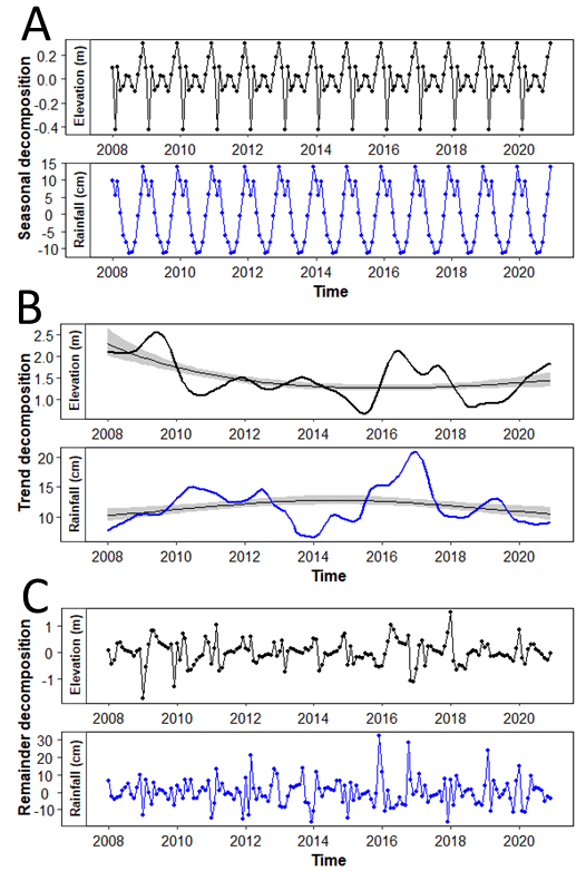
Trend analysis by use of the seasonal Mann-Kendall test was not significant for the maximum monthly rainfall time series from 2008 to 2021 (tau = –0.01, P = 0.10, n = 168), yet the time series for total monthly surface elevation showed a significant negative trend (tau = –0.34, P < 0.001, n = 168; Fig. 3B). Sen’s test was significant (z = –4.0, P < 0.001, n = 168, 95% CL = 0.00 to –0.002) with a slope of -0.004, which equates to a decrease in surface elevation at a rate of ~ -0.67 cm/month (n = 168 months) or ~ -6.7 cm over the 14-year period of the study. The correlation between plots of the decomposed trend components of surface lake elevation and rainfall was significant (r_s = 0.28, P = 0.001, n = 157) but not particularly strong. Pettitt’s test indicated that the probable change point in the decomposition of trend for lake elevation was April 2010 (k = row 28 in the data series; U* = 2,585, P < 0.001, n = 168). STL decomposition of the remainder or random term for monthly maximum lake surface elevation and rainfall showed highly erratic monthly sequences with large positive and negative spikes. The correlation between plots of decomposed random elements for surface lake elevation and rainfall was significant (r_s = 0.16, P = 0.04, n = 157; Fig. 3C) but the strength of the relationship was very weak.

Time series, Autocorrelation, and Diagnostics

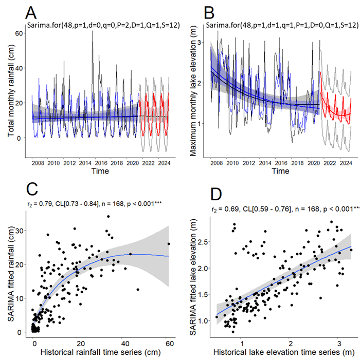
Visual assessment of each historical time series plot showed that an additive model was the most appropriate for each environmental attribute because variation remained relatively constant over time and did not depend on the level of the time series (Fig. 2A, 2B; Hyndman and ‎Athanasopoulos 2018). Autocorrelation and partial autocorrelation functions of the original data revealed that each time series model was significantly non-stationary as there were numerous autocorrelations lying outside the 95% confidence limits for both parameters; and the Box-test indicated that both data sets were significantly nonstationary (rainfall: ꭓ² = 233, df = 12, P < 0.001; lake surface elevation: ꭓ² = 161, df = 12, P < 0.001). Because each dataset showed strong seasonality and required differencing to become stationary best fit models were generated using the auto.arima function. Here both maximum non-seasonal and seasonal difference portions of ARIMA were set at 12 (i.e., maxd and maxD = 12, respectively).

This process resulted in a seasonal model forecasting rainfall (SARIMA[1,0,0] [2,1,1]12) and lake elevation (SARIMA [1,1,1] [1,0,1]12). Following this procedure, the Box-Pierce test using residuals for each SARIMA model was found to be not significant for each parameter as each P-value was > 0.05 indicating that the residuals were independent (rainfall: ꭓ² = 5.0, df = 12, P = 0.10; lake surface elevation: ꭓ² = 9, df = 12, P = 0.70). Thus, both models were considered stationary as verified with graphic illustrations (Appendix IIE and IIF (PDF)). These results indicated that the distribution of residuals in each time series was Gaussian (white noise), which: 1) statistically justified each proposed model, 2) demonstrated how an analysis of time series data may be done accurately, and 3) allowed continued processing of data with the ultimate goal of forecasting estimates of rainfall and lake elevation using SARIMA by use of the sarima.for function. 

Graphically, fitted values derived from each SARIMA model appeared relatively close to historical values (Fig. 4A and 4B). Analysis of the mean absolute percentage error (MAEP) showed that the average difference between the fitted model and the vector of historical rainfall was 68.6%. Whereas for lake elevation the average difference between vectors of the fitted model and the historical time series was 21.8%. Ranked correlation and GAM regression modes between fitted and historical values were significant for both rainfall and lake elevation (Fig. 4C and 4D), with percent deviance explained being almost identical in both comparisons (rainfall: F = 74.7, P < 0.001, R²(adj) = 0.460, DevExp = 38.7%; lake elevation: F = 50.8, P < 0.001, R²(adj) = 0.395, DevExp = 40.3%). As expected, the ranked correlation between the two fitted models of rainfall and lake elevation was significant (r_s = 0.32, P < 0.001, n = 168) and identical to the ranked correlation between each historical time series. The predictive power of each SARIMA model was illustrated graphically by forecasting 48 months-ahead of the time series for each environmental parameter (Fig. 4A). For both rainfall and surface lake elevation historical and fitted values for 2008 through 2021 were very similar. As expected, forecasted values for each time series model (surrounded by one-standard error) were also very similar to historical and fitted values. Results of modeling also suggested that forecasted lake levels will continue to show a declining trend in lake elevation into the future (Fig. 4B). 

Breaching

A representative breach event including variance in meteorological data for both terrestrial and marine attributes is illustrated by the permitted mechanical breach on 24 January 2020 (Fig. 5). The sequence of events in parameters surrounding this event is typical of conditions described by Kraus et al. (2008) and Pérez-Arlucea et al. (2011) for barrier beaches along the coast of northern California, in which a gradual rise in lagoon surface water increases the water-head difference between the lagoon and the ocean. During a “natural” breach overflow generally occurs at the narrowest section of the beach because increased rainfall and landscape runoff elevate the level of surface water to the edge of the sand berm. However, in the 24 January example the primary driver for the reduction in the level of water in the lagoon was the breach event. This act also prevented the possibility of weakening the sand barrier through seepage, which could have created a low elevation breach in the barrier beach typical of other such lagoon systems (Kraus 2008).

In the 24 January 2020 example, the relationship between rainfall and the surface lake elevation hydrograph was not particularly strong (r_s = 0.15, P = 0.005, n = 352; Fig. 5A, 5B, Fig. 6A). A multimodal distribution of HDRs (25%) was evident in the geometry of the GAM regression of daily rainfall versus lake elevation for the year, which included the breach event on the 24th (Fig. 6B). The highest concentration of HDR’s centered at ~1.6 cm of rainfall during the year as indicated by the red-colored points (probability = 50%), narrow width of the 95% confidence band of the regression, and the density of points in the rug along the x-axes (Fig. 6B). In contrast, the distribution of the next high density HDRs (dark-blue points, probability = 90%) were bimodal in their distribution during the ramp-up in intermediate levels of daily lake elevation and precipitation as the lagoon began to fill. Bimodality in the distribution of HDRs was evident in lake elevation > 3 m and rainfall > 2.5 cm leading up to breaching on 24 January. There were no high-density regions (light-blue colored points, probability > 95%) associated with the distribution of HDRs as surface elevation approached the breach event because breaching is a rare event and in 2020 it occurred only once. Further, except for lake elevation and wind direction, which shifted dramatically to the southwest (181° S, 263° W 4-days on either side of 24 January) at the time of the breach (210° SW), there were no other extrinsic meteorological climatic variables that exhibited a pattern suggesting that a natural breach was eminent had an artificial breach not occurred (Fig. 5C-H).

Historically at Lake Earl, most breach events (71.0%, n = 107) occurred in December (23.4%) and during the months of January (17.8%), February (15.9%), and March (14.0%) as predicted from the seasonal map (Fig. 2C and 2D). From 1987 to the present the average surface elevation of the lake at breaching was 2.79 m (1.3–3.4 m; n = 52; Table 2). From a univariate perspective the only variable that was significantly correlated with surface lake elevation was rainfall, but the strength of the relationship was extremely weak. As expected, wind speed, wind gust, and wave height were all significantly correlated as was wave height and dominant wave period (Table 2). Results of multiple regression analysis using GAM of variables observed at each breach event revealed that the proportion of both variance (55.0%) and null deviance (72.1%) explained by the rainfall + hightide + wave height suite of attributes was the “best” model with the lowest GCV statistic of all the other models evaluated (Table 3; Appendix IIIA–E (PDF)). Here, the proportion of the null deviance explained is probably more appropriate for non-normal errors (Wood 2017). Importantly, however, all models agreed that rainfall was the most significant predictive factor within each set of predictor variables modeled in the evaluation of surface lake elevation.    

Table 2. Basic statistics (Table 2a) and Spearman rank correlation coefficients (r_s; Table 2b) among environmental variables. ELV = lake surface elevation, RAF = rainfall, HTD = hightide, WDR = wave direction, WNS = wind speed, WGS = wind gust speed, WHT = wave height, and DWP = dominant wave period. Correlations are below the diagonal and probabilities (P-values) are above the diagonal; P = 0.5*, P = 0.01**, P = 0.001***

Table 2a. Basic statistics

Statistic	ELV	RAF	HAD	WDR	WNS	WGS	WHT	DWP
x̄	2.7	24.1	2.2	299.5	10.4	13.0	3.8	15.2
Min.	1.3	0.3	1.7	172.0	4.8	6.2	2.0	8.7
Max.	3.4	61.4	2.6	360.0	16.2	22.2	8.5	21.1
SD	0.4	13.6	0.3	74.3	3.4	4.3	1.4	3.2

Table 2b. Spearman rank coefficients

Variable	n	ELV	RAF	HAD	WDR	WNS	WGS	WHT	DWP
Lake surface elevation (m)	55	——	0.05*	0.74	0.75	0.75	0.75	0.24	0.18
Rainfall (cm)	42	0.30	——	0.56	0.50	0.76	0.76	0.96	0.61
Hightide (m)	37	-0.06	-0.10	——	0.62	0.64	0.68	0.37	0.27
Wave direction (deg)	32	-0.06	-0.12	0.09	——	0.48	0.33	0.11	0.23
Wind speed (m/s)	32	-0.06	-0.06	-0.09	-0.13	——	0.00***	0.06	0.52
Wind gust speed (m/s)	32	-0.06	-0.06	-0.08	-0.18	0.99	——	0.04*	0.34
Wave height (m)	31	-0.22	0.01**	0.17	-0.29	0.34	0.37	——	0.02*
Dominant wave period (sec)	31	-0.25	-0.10	0.21	-0.22	0.12	0.18	0.43	——

Table 3. Generalized Additive Model (GAM) multiple regression analyses for the suite of variables used to evaluate conditions surrounding breach events (GCV = generalized cross-validation). P = 0.5*, P = 0.01**, P = 0.001***

Variables	Estimated df	GAM-F	P-value
Rainfall (m)	2.52	5.41	0.005**
Hightide (m)	1.00	1.77	0.20
Wind direction (deg)	1.37	0.18	0.74
R2.adj.	32.0%	41.0%	n=32; GCV=0.029
Rainfall (m)	2.90	6.83	0.001***
Hightide (m)	1.00	2.29	0.14
Wind speed (m/sec)	3.47	1.16	0.39
R2.adj.	42.0%	54.0%	n=32; GCV=0.027
Rainfall (m)	2.81	6.41	0.002**
Hightide (m)	1.00	2.40	0.13
Wind gust (m/s)	2.20	1.07	0.41
R2.adj.	39.0%	49.0%	n=32; GCV=0.027
Rainfall (m)	2.74	7.56	0.001***
Hightide (m)	6.58	2.01	0.09
Wave height (m)	1.65	2.51	0.11
R2.adj.	55.0%	72.0%	n=31; GCV=0.027
Rainfall (m)	2.52	4.99	0.008**
Hightide (m)	1.00	0.79	0.38
Dominant wave period (sec)	1.00	0.92	0.35
R2.adj.	33.0%	41.0%	n=31; GCV=0.029

A comparison of the area and distribution of major vegetation communities found on LEWA shows that there has been both increases and decreases in the extent of different vegetation types between 2002 and 2014 (Fig. 7A and 7B). From the 2002 baseline to 2014 there has been: a 0.7% (18.6 ha) decrease in coastal dune habitat (i.e., foredune/beach strand), a 0.1% (2.1 hectare) decrease in coastal maritime forest habitat (i.e., upland trees/shrubs of spruce, grand fir, beach pine), a 1.1% (26.1 ha) increase in estuarine and brackish emergent marsh (i.e., aquatic plants at the lake periphery, floating, and rooted submergent species adapted to deeper lagoon waters), a 0.6% (13.7 ha) increase in forest and riparian wetland habitat (i.e., trees/shrubs tolerant of seasonal or temporary inundation during dormancy [winter] and saturated soils or high groundwater during growing season [summer]), a 1.3% (32.1 ha) decrease in freshwater emergent wetland and meadow habitats (i.e., herbaceous plants rooted in saturated or inundated soils that grow above water surface in non-estuarine conditions), and a 0.6% (13.9 ha) increase in grassland pasture (i.e., upland sandy soils dominated by grasses and forbs used for grazing purposes). I detected no noticeable increase in urban encroachment.

Discussion

Time Series Modeling of Rainfall

Descriptive statistics used in the analysis of rainfall and surface lake elevation showed that mean values of these parameters fluctuated dramatically, and both exhibited a distributional curve that was positively skewed and leptokurtic, particularly in lake elevation. Although seasonal Mann-Kendall and Sen’s slope statistics found no significant annual trend in precipitation, a significant annual trend was identified in surface elevation of lakes Earl and Tolowa from 2008 to 2021. Pettitt’s test suggested that the trend in decreasing surface elevation amounted to ~ 7.0 cm over the 14-year period of my study. STL decomposition and correlation analyses clearly showed that the decomposition factor that defined the most conspicuous difference between rainfall and surface elevation was the seasonal component followed distantly by the trend component. 

Seasonal time series analysis produced “best fit” models for each parameter with the lowest residual variance, AIC, BIC, and diagnostic checking criteria for both rainfall and lake elevation. Although the graphic presentation of fitted values produced by SARIMA appeared relatively close to the historical values for each environmental parameter, the mean average difference (MAEP) between the fitted model and the vector of historical data was smallest for surface lake elevation. This finding suggests that SARIMA for surface lake elevation is reasonably stable with only minor structural differences compared to historical values. The difference between models also suggests that SARIMA for surface lake elevation is potentially better at forecasting future values than is the SARIMA for rainfall in forecasting precipitation. A poor fit by SARIMA for rainfall may reflect the more stochastic nature of the “natural” precipitation regime, as opposed to a regular and systematically implemented mechanical breaching program post 2000. In either instance, generally but not always, as the period between the date of forecast and the actual forecast period narrows there also will be a corresponding reduction in model error for both parameters, in this case beyond a 36-to-48-month period.

Individual Breaching Events

GAM regression of historical rainfall and surface lake elevation in combination with a recent case history of daily and monthly rainfall and lake elevation for the year 2020 suggested that the relationship between direct precipitation and surface lake elevation was not highly correlated in the ramp-up to annual breach events. Given that there was no trend in rainfall for the years I evaluated, it is not reasonable to hypothesize that climate change was responsible for the amount of direct seasonal precipitation into the lakes. A more likely explanation is that the amount of water entering Lake Earl from the surrounding landscape and regional watershed decreased in association with evaporation, which in fact could be related to climate change. For example, the United States Geological Survey estimates evaporation in Humboldt-Arcata Bay to the south to be ~0.76 m annually (Meyers and Nordenson 1962). Alternatively, the amount of water retained seasonally in the lake and lagoon system may simply be a function of the systematic breaching program initiated in earnest in the 1990’s (Anderson 2002; Anderson and Schlosstein 2003; CDFG 2003; Low 2003). Exceedance of the current breaching threshold would tend to decrease the slope of the regression line resulting in the trend I documented. Moreover, it seems reasonable to assume that the potential moderating effect of regular seasonal breaching and the duration of time that the breach stayed open would result in fewer high surface elevations compared to historical natural breach events or those associated periods when the area was less populated immediately adjacent to Lake Earl.

Natural and manual breaching of barrier beach lagoons holds consequences for species transiting or inhabiting freshwater-brackish lake and lagoon systems (Kraus et al. 2008). However, the ecological impacts to native plant and animal communities as a function of flooding by not breaching the sand barrier annually have not been studied. Results of my mapping analysis of vegetation within the LEWA suggests that increases in estuarine and brackish emergent marsh, forest-riparian wetland habitat, and grassland pasture, coupled with a decrease in freshwater emergent wetlands is consistent with a reduction in surface lake elevation and vegetation encroachment. Moreover, observations of degraded patches of Sitka spruce and beach pine (i.e., coastal maritime forest habitat) have recently been identified at surface elevations that occasionally exceed the threshold for breaching (> 2.5 m) in areas peripheral to Lake Earl (F. Kemp, pers. comm. 2022). This observation also may signal encroachment of vegetation as a function of reduced rainfall and inflow from the landscape suggestive of shrinkage in total acreage of wetland habitat types. 

However, my hypothesis that vegetation encroachment may be a function of regular breaching at permitted seasonal levels of surface elevation remains to be evaluated by use of updated ground-truth vegetation and species-specific plant surveys, in conjunction with GIS digital mapping, and statistical quantification. Additionally, vertical land motion in Crescent City appears to be uplifting at ~0.3 cm/year, or ~4.2 cm over the course of my 14-year study (J. Anderson, pers. comm. 2022). Anderson further notes that because the vertical land movement is upward, it’s in the opposite direction of the decreasing trend in lake level reported herein. Thus, the combined lake level may have decreased ~11 cm over 14 years.

Based on the forecasted estimates of a reduced seasonal pattern of lake levels and the trends in vegetation communities that I document, there may be a potential threat to desirable freshwater and brackish wetland habitats in the surrounding terrestrial landscape. This eventuality could impact wildlife inhabiting or transiting the connected coastal lake and lagoon ecosystem and overall biological diversity of the wildlife area as a function of systematic breaching of the lagoon system. Similarly, the statement that an increase in the maximum surface elevation of Lake Earl would facilitate greater flexibility in the implementation of management objectives and benefit ecological objectives (Anderson 2002) would benefit from the identity of what specific ecosystem processes, functions, and benefits would derive from such a policy.

Importantly, my analysis did not evaluate the seasonal long-term effects of: 1) hydrological factors such as input into the lake-lagoon system attributable to runoff from the landscape, 2) accumulation of lake sediment or marine sand; 3) hydrological events associated with water displacement and geomorphological changes in the architecture of the sandy barrier beach, 4) differences in head pressure between the lagoon and the barrier beach, 5) geomorphological processes associated with the buildup of the sand barrier between the lagoon and the ocean; or 6) infiltration of salt water from marine sources including wave-over wash. Although these factors are briefly discussed individually for the Lake Earl-Tolowa lagoon system elsewhere (Anderson 2002; Anderson and Schlosstein 2003; Lowe 2003; Kraus et al. 2008), they await detailed data gathering, analysis, and groundwater/hydrologic/lake modeling in order to truly understand the dynamic physical process and relationship between terrestrial, lake-lagoon, and marine ecosystem structure and function upon which management depends. Nevertheless, results of multiple regression provided additional insight into several extrinsic factors in the run-up to breaching that have not previously been evaluated. For example, despite the issue of small sample size, GAM modeling identified a “best” fit model based on a combination of rainfall, hightide, and wave height as a function of the percentage of variance explained in the regression. Further, all GAM models indicated that rainfall was the most significant predictive factor within each set of predictor variables modeled in evaluating surface lake elevation, although the relationship was not particularly strong.

Recommendations

There is no debate that the lakes Earl-Tolowa lagoon ecosystem is complex, dynamic, and governed by extreme variance in environmental variables (Anderson 2002; Anderson and Schlosstein 2003). Therefore, this study is germane to the management of LEWA and associated wetland habitat surrounding the area for wildlife policy implications. Results of my study suggest a more detailed analysis including a combination of climatological, hydrological, and geomorphological analyses and modeling, encompassing both terrestrial and marine environments surrounding the lake and lagoon system is needed to fully understand the short-and long-term dynamic process of this lake-lagoon function. Knowledge of this depth and scope is critical to effective and efficient management of terrestrial and aquatic diversity and resource planning at the LEWA. For example, Kraus et al. (2008) stressed that: 1) there is much that can be learned about barrier breaching from the lagoon side through site-specific monitoring; and 2) more detailed data-driven and long-term evaluation of the “susceptibility index” cannot be taken as general because it relates to the specific wave and littoral regime, tide range, and sediment supplies responsible for building the sand barrier beach. 

Further, this deficit in knowledge contributes to the underestimation of modeling due to perturbations in the process as a function of manual breaches prior to the water level in the lagoon reaching a level to cause overflow, and increased seepage under a natural breaching regime. Taylor and Frobel (2003) suggest the need to document by use of morphological evidence the seasonal pattern and importance of wave scour of the sand barrier during the process of natural breaching of the barrier. The wave-driven dynamics of the Tolowa lagoon differs markedly from fluvial-driven dynamics described by Kirk (1991). Given that there is a gradation in the relative influence of marine versus fluvial processes in different lake-mouth lagoon environments, with the balance between these two agents affecting the types and frequencies of changes occurring, more information is needed to evaluate the significance of marine processes. 

Similarly, management of the LEWA in the context of natural resource planning, future climate change, and sea level rise in relation to continued breaching of the lagoon also depends upon understanding the dynamic underpinnings of the lake-lagoon ecosystem. Increasingly encroachment of utilities associated with the civilian community are impacted if the surface elevation of the lake becomes too high and the lagoon is not manually breached to prevent flooding of adjacent private property and infrastructure, and to potentially improve water quality of the lagoon (Wamsley et al. 2007). At some sites, especially along the coast of California, biologists have attempted to evaluate the best season and conditions for breaching to replicate and maintain the natural ecological functioning of the system (Hofstra and Sacklin 1987). However, studies have not been performed at lakes Earl and Tolowa to warrant breach events that optimize maintenance of “natural” ecological functioning of the lagoon system, but instead have focused on the need for breaching to address issues related to flooding of utilities and water quality. 

Some specific questions remain: 1) What are the data to evaluate how often breaching occurs from the lagoon side and how often it occurs from the ocean side? 2) How important is movement of sediment through the lake-lagoon system in formation of a barrier compared to movement of sand from the ocean side? 3) What is the primary source of sand that forms the beach barrier from the ocean side of the lagoon? 4) How often do waves breach the barrier directly from ocean to lagoon or is there sufficient raised lagoon water levels beyond that which the barrier could support, inducing a breach via pipe failure from lagoon to sea as the hydraulic head between the lagoon and sea increases on the falling tide? 5) What happens when the inlet is closed in relation to changes in elevation in the lagoon due to marine tides and water interchange via phreatic leaking during months of fall-winter hightides? 6) What is the role and importance of upper phreatic zones in sustaining biological diversity in the terrestrial, lake, and lagoon ecosystems because some plant and animal species fully depend upon the lake level and quality (Abdullah et al. 1997; Hart 2007)? 7) What affect does estimates of vertical land movement have on lake and lagoon levels? 8) What is the offshore configuration of the marine bottom topography that would create wave deflection?

These and other hydrological, ecological, and biological questions have not been evaluated and are needed in assessing the importance of barrier formation through natural processes. Use of monthly and hourly time-lapse digital photography could be used to evaluate many of the processes associated breaching at the mouth of the Tolowa lagoon. This methodology would allow better understanding of the dynamic forces behind the lake-lagoon-breach process and morphological reconfiguration of the mouth of the lagoon that accompany such forces. Understanding the driving cycles of lagoon behavior from closure to breaching requires additional knowledge that currently is unavailable. As such, specific long-term site-specific management actions could include daily documentation and monitoring of: 1) morphological and architectural changes, and equilibrium states of the sand barrier prior to a breach event, storm surge, storm-wave behavior, wave overtopping of the sand barrier, and high-tide events, and outlet channel dynamics (widening, migration, truncation); 2) ground water, surface water, and lagoon water fluctuations, and extent of flood events in the surrounding landscape; 3) precipitation, and surface lake elevation on site; 4) monthly measurements of surface water temperature and estimates of lake and lagoon evaporation; 5) monthly sediment deposition/accretion within the lagoon; 6) fluctuations in lake-lagoon salinity levels and relevant water quality metrics; and 7) update plant species surveys and GIS-based vegetation mapping for the entire LEWA.

Acknowledgments

Many thanks to Dr. Robert Hyndman and S. Gupta with regard to the use of high-density region analyses. I thank several anonymous reviewers for their helpful editorial comments, suggestions, and numerous probing questions, which in several instances will require future research to address them. I am particularly appreciative of Jeffrey K. Anderson (Northern Hydrology, McKinleyville, California) for providing a critical review of this manuscript, making valuable suggestions on content, and for allowing use of his estimates of vertical land movement as relates to Lake Earl.

Literature Cited

• Abdullah, M. H., M. B. Mokhtar, S. H. J. Tahir, and A. B. T. Awaluddin. 1997. Do tides affect water quality in the upper phreatic zone of a small oceanic island, Sipadan Island, Malaysia? Environmental Geology 29:112–117.
• Akaike, H. 1973. Information theory and an extension of the maximum likelihood principle. Pages 267–281 in B. N. Petrov and F. Csáki, editors. 2nd International Symposium on Information Theory, Tsahkadsor, Armenia, Budapest, USSR.
• Anderson, J. K. 2002. Lake Earl and Lake Tolowa hydrologic review/analysis. Final Technical Memorandum, Grahm Matthews and Associates, Weaverville, CA, USA.
• Anderson, J. K., and B. Schlosstein. 2003. Appendix B – Hydrologic analysis, in Lake Earl management plan – draft environmental Impact report, California Department of Fish and Game, Sacramento, CA, USA
• Box, G. E. P., and G. M. Jenkins. 1970. Time Series Analysis: Forecasting and Control. Holden-Day, San Francisco, CA, USA.
• Burnham, K. P., and D. R. Anderson. 1998. Model Selection and Inference: A Practical Information-Theoretic Approach. Springer-Verlag, New York, NY, USA.
• California Department of Fish and Game (CDFG). 2003. Lake Earl Management Plan Environmental Impact Report (EIR). California Department of Fish and Game, Eureka, CA, USA.
• Cleveland, R. B., W. S. Cleveland, J. E. McRae, and I. Terpenning. 1990. STL: a seasonal-trend decomposition procedure based on Loess. Journal of Official Statistics 6:3–73.
• Cleveland, W. S., E. Grosse, and W. M. Shyu. 1992. Local regression models. Pages 309–376 in J. M. Chambers and T. Hastie, editors. Statistical Models in S. Chapman and Hall, New York, NY, USA.
• Corder, G. W., and D. I. Foreman. 2014. Nonparametric Statistics: A Step-by-step Approach. John Wiley and Sons, Inc., Hoboken, NJ, USA.
• Delignette-Muller, M. L., and C. Dutang. 2015. fitdistrplus: an R package for fitting distributions. Journal of Statistical Software 64:1–34.
• Diankha, O., and M. Thiaw. 2016. Studying the ten years variability of Octopus vulgaris in Senegalese waters using generalized additive model (GAM). International Journal of Fisheries and Aquatic Studies 2016:61–67.
• Dimri, T., S. Ahmad, and M. Sharif. 2020. Time series analysis of climate variables using seasonal ARIMA approach. Journal of Earth System Science 129:1–16.
• Fuller, W. A. 1976. Introduction to Statistical Time-series. John Wiley and Sons, Inc, Hoboken, NJ, USA.
• Gilbert, R. O. 1987. Statistical Methods for Environmental Pollution Monitoring. John Wiley and Sons, Inc, Hoboken, NJ, USA.
• Hart, D. E. 2007. River mouth lagoon dynamics on mixed sand and gravel barrier coasts. Journal of Coastal Research, Special Issue 50:927–931.
• Hastie, T., and R. Tibshirani. 1990. Generalized additive models. Statistical Science 1:297–301.
• Helsel, D. R., R. M. Hirsch, K. R. Ryberg, S. A. Archfield, and E. J. Gilroy. 2020. Statistical Methods in Water Resources. U.S. Geological Survey, Techniques and Methods Book 4, Chapter A3. https://doi.org/10.3133/tm4a3
• Hill, T., and P. Lewicki. 2007. Statistics: Methods and Applications. StatSoft, Tulsa, OK, USA.
• Hipel, K. W., and A. I. McLeod. 2005. Time series modelling of water resources and environmental systems. Developments in Water and Science 45. Elsevier, Amsterdam, Netherlands.
• Hirsch, R. M., J. R. Slack, and R. A. Smith. 1982. Techniques for trend assessment for monthly water quality data. Water Resources Research 18:107–121.
• Hofstra, T. D., and J. A. Sacklin. 1987. Restoring the Redwood Creek estuary. Pages 812–825 in O. T. Maggon, edtior. Coastal Zone ’87: Proceedings of the Fifth Symposium on Costal and Ocean Management. American Society of Civil Engineers, Seattle, WA, USA.
• Hyndman, R. T. 1996. Computing and graphing highest density regions. The American Statistician 50:120–126.
• Hyndman, R. J., and Y. Khandakar. 2008. Automatic time series forecasting: the forecast package for R. Journal of Statistical Software 26.
• Hyndman, R. J., and G. Athanasopoulos. 2018. Forecasting: Principles and Practice. 2nd edition, OTexts, Melbourne, Australia.
• Johnson, J. W. 1976. Closure conditions of northern California lagoons. Shore and Beach 44:20–24.
• Kendall, M. G. 1975. Rank Correlation Methods. 4th edition. Charles Griffin, London, UK.
• Kirk, R. M. 1991. River-beach interaction on mixed sand and gravel coasts: a geomorphic model for water resource planning. Applied Geography 11:267–287.
• Kraus, N. C., A. Militello, and G. Todoroff. 2002. Barrier breaching processes and barrier spit breach, Stone Lagoon, California. Shore and Beach 70:21–28.
• Kraus, N. C., K. Patsch, and S. Munger. 2008. Barrier beach breaching from the lagoon side, with reference to Northern California. Shore and Beach 76:33–43.
• Lauck, D. R. 1997. 1997 studies of the Oregon silverspot butterfly (Speyeria zerene hippolyta) and the host violets (Viola adunca and Viola langsdorffii) near Lake Earl in Del Norte County, California. Report to Pacific Shores Water District, Crescent City, CA, USA.
• Lewis, C. D. 1982. Industrial and Business Forecasting Methods. Butterworths, London, UK.
• Ljung, G. M., and G. E. P. Box. 1978. On a measure of lack of fit in time series models. Biometrika 65:297–303.
• Lowe, J. 2003. Management of Lake Earl lagoon water elevations: PWA hydrology study conclusions. Philip Williams and Associates, San Francisco, CA, USA.
• Machiwal, D., and M. K. Jha. 2006. Time series analysis of hydrological data for water resources planning and management: a review. Journal of Hydrology and Hydromechanics 54:237–257.
• Madsen, H., and P. Thyregod. 2011 Introduction to General and Generalized Linear Models. Chapman and Hall/CRC, Boca Raton, FL, USA.
• Mann, H. B. 1945. Non-parametric tests against trend. Econometrica 13:163–171.
• Martínez-Acosta, L., J. P. Medrano-Barboza, Á. López-Ramos, J. F. R. López, and A. A. López-Lambraño. 2020. SARIMA approach to generating synthetic monthly rainfall in the Sinú River watershed in Colombia. Atmosphere 112:16.
• Meyers, J. S., 1962. Evaporation from the 17 Western States. U.S. Geological Survey Professional Paper 272-D, Washington, D.C., USA. Available from: https://pubs.usgs.gov/pp/0272d/report.pdf (PDF)
• McDonald, J. H. 2014. Handbook of Biological Statistics. Sparky House Publishing, Baltimore, MD, USA.
• Moreno, J. J. M., A. P. Pol, A. S. Abad, and B. C. Blasco. 2013. Using the R-MAPE index as a resistant measure of forecast accuracy. Psicothema 4:500–506. https://www.redalyc.org/pdf/727/72728554013.pdf (PDF)
• Nau R. 2017. ARIMA models for time series forecasting. Statistical Forecasting: Notes on Regression and Time Series Analysis. Available from: https://people.duke.edu/~rnau/411home.htm
• Nicholls, N. 2012. Is Australia’s continued warming caused by drought? Australian Meteorological and Oceanographic Journal 62:93–96.
• Nychka. 1988. Bayesian confidence intervals for smoothing splines. Journal of the American Statistical Association 83:1134–1143.
• O’Hara-Wild, M., S. Pearce, R. Nakagawara, S. Gupta, D. Vanichkina, E. Tanaka, T. Fung, and R. Hyndman. 2022. gghdr: visualisation of highest density regions in ‘ggplot2’. R package, version 0.1.0. Available from: https://github.com/Sayani07/gghdr/
• Papalaskaris, T., T. Panagiotidis, and A. Pantrakis. 2016. Stochastic monthly rainfall time series analysis, modeling and forecasting in Kavala city, Greece, North-Eastern Mediterranean Basin. Procedia Engineering 162:254–263. 
• Papalaskaris, T. and G. Kampas. 2017. Time series analysis of water characteristics of streams in Eastern Macedonia–Thrace, Greece. European Water 57:93–100.
• Pérez-Arlucea, M., C. Almécija, R. González-Villanueva, and I. Alejo. 2011. Water dynamics in a barrier lagoon system: controlling factors. Journal of Coastal Research, SI 64 Proceedings of the 11th International Coastal Symposium:15–19. 
• Schwarz, G. 1978. Estimating the dimension of a model. Annals of Statistics 6:461–464.
• Sen, P. K. 1968. Estimates of the regression coefficient based on Kendall’s tau. Journal of the American Statistical Association 63:1379–1389.
• Shumway, R. H., and D. S. Stoffer, 2017. Time Series Analysis and Its Applications: With R Examples. 3rd edition. Springer Texts in Statistics. Springer, New York, NY, USA.
• Smith, G. L., and G. A. Zarillo. 1988. Short-term interactions between hydraulics and morphodynamics of a small tidal inlet, Long Island, New York. Journal of Coastal Research 4:301–314.
• Stephens, M. A. 1979. Test of fit for the logistic distribution based on the empirical distribution function. Biometrika 66:591–5.
• Stoffer, D. S., and R. H. Shumway. 2019. Time Series: A Data Analysis Approach Using R. Chapman and Hall, London, UK.
• Sullivan, R. M., and J. P. Hileman. 2020. Time series modeling and forecasting of a highly regulated riverine system: implications for fisheries management. California Fish and Wildlife Journal 106:221–259.
• Taylor, R. B., and D. Frobel. 2003. Rapid transformation of upper beach characteristics along breached coastal barriers, Atlantic Nova Scotia. Proceedings of the Canadian Coastal Conference, Kingston, Ontario, Canada.
• Tetra Tech. 2000. Intensive habitat study for Lake Earl and Lake Tolowa, Del Norte County, California. Tetra Tech, Inc., Final Report to the USACE, San Francisco District, San Francisco, CA, USA.
• Tsiatis, A. A. 2006. Semiparametric Theory and Missing Data. Springer Texts in Statistics. Springer, New York, NY, USA.
• Wamsley, T. V., N. C. Kraus, M. Larson, H. Hanson, and K. J. Connell. 2007 Pages 2818–2830 in J. M. Smith, editor. Coastal barrier breaching: comparison of physical and numerical models. Proceedings of the 30th Coastal Engineering Conference. World Scientific Press, San Diego, CA, USA.
• Wang, X., K. S. Smith, and R. J. Hyndman. 2006. Characteristic-based clustering for time series data. Data Mining and Knowledge Discovery 13:335–364.
• Wood, S. N. 2017. Generalized Additive Models: An Introduction with R. 2nd edition. Chapman and Hall/CRC Press, London, UK.

¹ https://www.ncdc.noaa.gov/cdo-web/datasets/GHCND/stations/GHCND:USW00024286/detail (rainfall)

² https://cdec.water.ca.gov/dynamicapp/staMeta?station_id=EFD (lake elevation)

³ https://tidesandcurrents.noaa.gov/historic_tide_tables.html (high tide data 2008–2021)

⁴ https://tidesandcurrents.noaa.gov/noaatidepredictions.html?id=9419750 (high tide data 2000–2007)