FULL RESEARCH ARTICLE

Thomas Connor^1,2, Thomas J. Batter², Cristen O. Langner³, Jeff Cann⁴, Cynthia McColl⁵, and Richard B. Lanman^5,6*

¹ University of California, Berkeley, Department of Environmental Science, Policy, and Management, 130 Mullford Hall #3114, Berkeley, CA 94720, USA  https://orcid.org/0000-0002-7630-5156
² California Department of Fish and Wildlife, Wildlife Branch, Game Conservation Program, 1010 Riverside Parkway, West Sacramento, CA 95605, USA https://orcid.org/0000-0002-3957-3725
³ California Department of Fish and Wildlife, Central Region, 1234 E Shaw Avenue, Fresno, CA 93710, USA
⁴ California Department of Fish and Wildlife, Central Region, 20 Lower Ragsdale Drive, Suite 100, Monterey, CA 93940, USA
⁵ North Santa Clara Resource Conservation District, 1560 Berger Drive, Room 211, San Jose, CA 95112, USA
⁶ Institute for Historical Ecology, 556 Van Vuren Street, Los Altos, CA 94022, USA https://orcid.org/0000-0001-8122-4329

*Corresponding Author: ricklanman@gmail.com

Published 29 December 2023 • doi.org/10.51492/cfwj.109.19

Abstract

While California’s statewide tule elk (Cervus canadensis nannodes) population has recovered from two or three individual survivors in the late 19th century, the subspecies exists today in numerous widely disjunct populations, leaving vast areas of the species’ former range uninhabited. Large unoccupied areas of historic tule elk range include the Santa Cruz Mountains and the northern Diablo and northern Santa Lucia ranges. Natural range expansion by existing populations into these areas is blocked by major highways and urban development; although, before considering tule elk translocations, it is necessary to assess the habitat suitability there. To this end, we fit a resource selection function (RSF) using generalized linear mixed models to GPS collar data collected from nearby radio collared tule elk and used several environmental GIS layers to capture important habitat characteristics. We fit the RSF in a habitat use versus availability framework with only linear and quadratic terms and used stepwise model selection ranked by AICc to maximize its generalizability, enabling transferability to our unoccupied study area. We also used k-fold cross validation to evaluate our RSF and found it predicted habitat within the San Luis Reservoir herd well. The fit habitat relationships mostly followed expectations based on tule elk ecology, including positive responses to herbaceous vegetation cover and waterbody proximity, and negative responses to high tree cover and high puma habitat suitability. Our RSF accurately predicted currently occupied elk habitat as suitable and found well over 500,000 ha (2,000 mi²) of suitable but unoccupied habitat throughout the northern Diablo Range, the inland and coastal sides of the Santa Cruz Mountains, and the northern Santa Lucia Range. Assuming translocations, and construction and improvement of highway wildlife crossings, our results support the potential for re-establishing tule elk in these regions, which are more coastal and mesic than the species’ current habitat in the central Diablo and northern Gabilan ranges.

Key words: Cervus canadensis nannodes, elk, habitat suitability, restoration, tule elk

Citation: Connor, T., T. J. Batter, C. O. Langer, J. Cann, C. McColl, and R. B. Lanman. 2023. Habitat suitability assessment for tule elk in the San Francisco Bay and Monterey Bay areas. California Fish and Wildlife Journal 109:e19.

Editor: Karen Converse, Wildlife Branch

Submitted: 6 June 2023; Accepted: 12 September 2023

Copyright: ©2023, Connor et al. This is an open access article and is considered public domain. Users have the right to read, download, copy, distribute, print, search, or link to the full texts of articles in this journal, crawl them for indexing, pass them as data to software, or use them for any other lawful purpose, provided the authors and the California Department of Fish and Wildlife are acknowledged.

Competing Interests: The authors have not declared any competing interests.

Introduction

Elk (Cervus canadensis) are California’s largest land animal and native grazer (CDFW 2018). Of the five subspecies of elk in North America, three are native to California, but only the tule elk (C. c. nannodes) is endemic (Meredith et al. 2007). California’s statewide tule elk population is presently fragmented into more than 20 separate populations, with generally poor connectivity between them (CDFW 2018; Batter et al. 2021). Habitat fragmentation increases vulnerability to inbreeding depression, and for tule elk this is especially concerning due to this subspecies’ rapid decline and the resulting extreme genetic bottleneck in the 1860s. Landscape change was a major influence in the tule elk decline that began during Spanish colonization and was accelerated by Anglo-American occupancy after the 1849 gold rush (McCullough 1969). Introduction of exotic plants, competition with confined and feral livestock, disruption of aboriginal fire practices, unregulated market and sport hunting, conflict with agriculture, and other human developments have had profound ecological impacts on tule elk abundance and distribution and the landscapes they rely upon (van Dyke 1902; Burcham 1957; Thompson 1961; McCorriston 1994; McCullough et al. 1996). Despite a ban on hunting imposed in 1854 (CDFG 1928; McCullough et al. 1996) the population crashed, and by 1870 was restricted to the remnant tulemarshes of the southern San Joaquin Valley. By 1873 tule elk were thought to be extinct. Then in 1874, two or three individuals were discovered near Buttonwillow and were afforded protection by cattleman Henry Miller on his Kern County ranch (Evermann 1915; McCullough 1969). Recent genetic studies support this narrative, indicating that all contemporary tule elk are descended from two or three individuals (Sacks et al. 2016).

Through translocations and legal protections, the statewide tule elk population has increased, and now numbers over 6,000 individuals (CDFW 2018; Batter et al. 2021). Translocations have played a critical role in tule elk recovery, occurring in two general phases (McCullough et al. 1996). The initial phase was prompted by significant growth and agricultural damage committed by the protected remnant population on the Miller and Lux Ranch. These translocations occurred between 1904 and 1933 and were primarily led by the U.S. Biological Survey and the California Academy of Sciences. Most of the reintroduction efforts ultimately failed to establish permanent herds, generally due to inadequate numbers being translocated to a given site (Evermann 1916) or human-wildlife conflicts leading to elk being shot or relocated (McCullough 1969). The elk’s primary predators, the grizzly bear (Ursus arctos horribilis) and gray wolf (Canis lupus), were unlikely culprits as they were extirpated from California by 1924 (Fry 1924) and 1922 (Grinnell 1933), respectively. The exceptional successes were the establishment of a permanent population in Colusa County in 1922 and in the Owens Valley in Inyo County in 1933, the latter beyond the recognized historical range east of the Sierra Nevada (McCullough 1969; Dasmann 1975; Watt 2015). Some elk remained on the Miller and Lux ranch in a wild state during these events, but subdivision of the property and increasing complaints of crop damage necessitated further action. In 1934, the remaining elk in this location were captured and placed within a fenced tract of land set aside as an elk refuge (Dasmann 1975; McCullough 1969). Translocations ceased until opposition to controlled hunts of the Inyo County population brought renewed public interest towards tule elk recovery (McCullough et al. 1996). In 1971, California State Senate Bill 722, known as the Behr bill, targeted expansion of the state’s 600 tule elk to at least 2,000, and, in 1976, Congress passed a joint resolution, Public Law 94-389, which required the secretaries of defense, agriculture, and the interior to cooperate with the state in making suitable federal lands reasonably available for tule elk. This legislation spurred the California Department of Fish and Game to translocate elk from the mid-1970s to 1998 to over 20 locations (CDFW 2018).

Although periodic translocations have continued to occur using captive herds as sources to augment established free-ranging populations, no translocations have been initiated to establish new metapopulations for 25 years (CDFW 2018; Batter et al. 2021). Although the California Department of Fish and Wildlife (CDFW) Elk Management Plan asserts that “much of the historical suitable habitat now supports elk”, it also states that “future management efforts will likely involve translocation of surplus elk to improve the status of an existing population, maintain or increase genetic interchange between isolated populations and to recolonize elk to their historical ranges” (CDFW 2018). Although elk populations continue increasing in both distribution and abundance in California, fragmented habitat precludes functional connectivity (demographic and genetic exchange) across many populations. This also prevents dispersal to and occupancy of suitable habitat that could foster additional population growth and redundancy. Changing habitat conditions and continued human alterations across landscapes pose a threat to elk population persistence, thus necessitating an assessment of existing unoccupied and potentially suitable habitat. For example, an aerial survey of the eastern Santa Clara County elk herds found an unexpectedly meager growth rate over the last 40 years, consistent with other studies suggesting that linkages to unoccupied but more mesic regions may be critical to future tule elk resilience (Denryter and Fischer 2022; Lanman et al. 2022a). Where unoccupied suitable habitat exists, it presents an opportunity for wildlife and land managers to identify potential sites for highway crossings, promote natural or artificial landscape connectivity, and reexamine translocation as a tool to restore elk on the landscape. The return of elk to unoccupied patches, whether through development of wildlife crossings across traffic infrastructure barriers or human-assisted translocations, may have added ecological benefits such as restoration of desirable ecosystem function, provision of desirable wildlife viewing opportunities (USFWS 2012), and grazing to reduce fire fuel loads (LeComte et al. 2019; Defrees et al. 2020). The latter is particularly important in California as wildfires have doubled in frequency since the 1980s (Goss et al. 2020) and are principally driven by increasing aridity and high understory fire fuel load biomass (Potter and Alexander 2022).

Tule elk herd home range size requirements decrease dramatically nearer the coast where more mesic habitat promotes forage and water availability (Lanman et al. 2022a). Thus, highway crossings or translocations enabling elk to range closer to the Pacific Ocean may bolster resilience of tule elk populations in the face of California’s progressively warmer and more arid climate (Williams et al. 2020). In particular, the Santa Clara-Mt. Hamilton and Alameda Elk Management Units (EMUs) in the Central Diablo Range are expected to be moderately vulnerable (i.e., likely to experience a decrease in abundance or range extent) to climate change by mid-century (Denryter and Fischer 2022). Tule elk were historically common in the more coastal San Francisco Bay and Monterey Bay regions during pristine conditions but were extirpated by the 1850s (Evermann 1915; McCullough 1969).

Today, the Santa Cruz Mountains and north Diablo Range regions, in the west, south, and east San Francisco Bay areas, respectively, are relatively unique in the nation in terms of high percentages of protected lands near major metropolitan areas, with 28% and 29% of total area protected, respectively (Bay Area Open Space Council 2019). Monterey County, which subsumes the north Santa Lucia Range, has a much greater volume of protected lands than the former counties, but less as a percentage of total land area at 21% (AECOM 2021). These protected lands are managed by federal, state, county, and local special districts and may have significant public access and recreation. Elk in general avoid all-terrain vehicle riding on trails similarly to motorized traffic, with intermediate avoidance of mountain biking, and less avoidance of hiking and horseback riding, although the tule elk subspecies is not specifically well studied in this regard (Wisdom et al. 2018). Anecdotally, tule elk have highly varying tolerances of human presence, possibly related to the degree of exposure to and type of human activity (Phillips 2023).

The protected and conserved lands nearer the coasts of San Francisco and Monterey bays offer cooler and more mesic habitats with much smaller tule elk home range size requirements of 217 ha (536 acres) at Point Reyes and 401 ha (991 acres) at Mt. Hamilton (Cobb 2010; Duncan 1988). By comparison, tule elk herds in more arid regions such as the Owens Valley or Carrizo Plain require more than an order of magnitude more land (Lanman et al. 2022a). Much of the protected land in the Santa Cruz Mountains and Santa Lucia Range are dense forest unsuitable for tule elk, which have high affinity for grasslands, chapparal, and open woodlands (McCullough 1969). Additionally, patch size alone is not indicative of quality elk habitat. To better understand if and to what extent suitable habitat exists in this area, a detailed habitat suitability analysis for tule elk is needed which can then be used to inform management actions including potential for translocations, habitat enhancement, construction of freeway overcrossings, and/or improvement of existing undercrossings (Lanman et al. 2022b).

To assess habitat suitability of an area that is unoccupied by tule elk, it is necessary to use the habitat selection patterns of other nearby tule elk populations to make empirical evaluations about available habitat in the Santa Cruz Mountains and wider regions. The nearest extant tule elk herd with contemporary collar data is in eastern Santa Clara County and western Merced County around San Luis Reservoir. Elk from these populations were GPS-collared as part of a separate study to assess home range and habitat use. We leveraged this existing telemetry dataset to generate resource selection functions fit with logistic regression and projected the resulting model to predict tule elk habitat suitability in presently unoccupied range throughout the Santa Cruz Mountains, north Diablo Range, and north Santa Lucia Range regions.

Methods

Study Area

We assessed the suitability of the Santa Cruz Mountains region, consisting of San Mateo, Santa Cruz, and western Santa Clara counties, the northern Diablo Range region, consisting of Contra Costa, Alameda, and eastern Santa Clara counties, and the northern Santa Lucia Range region, consisting of Monterey County. These regions contain large areas of protected lands but remain inaccessible to elk unless wildlife crossings or translocations enable them to cross major highway infrastructure (Fig. 1).

The Santa Cruz Mountain range is a 141 km (71 mi) chain of coastal mountains stretching from Montara Mountain in the north, to the Pajaro River in the south (Thomas 1975). West and south of San Francisco Bay the Santa Cruz Mountains provide temperate, wet conditions on the coastal side and drier conditions on the inland side. Average temperatures are approximately 10 °C in winter and 20 °C in summer. There is an average of 60 cm precipitation, mostly in winter (October–March), with an east-west annual precipitation gradient of 48 cm in Coyote Valley and 78 cm in Santa Cruz. Common vegetation communities in the region include grassland, chaparral, oak (Quercus spp.) woodland, oak and mixed coniferous woodland, coast redwood (Sequoia sempervirens) forest, and wetland (Stephens and Fry 2005). These floral communities transition from coastal grassland near the Pacific Ocean, to mixed coast redwood and Douglas fir (Pseudotsuga menziesii) at higher elevations. On the inland side, the coniferous forest transitions to oak woodland and chaparral at lower elevations.

The Diablo Range is a 314 km (195 mi) chain of inner coast range mountains beginning at Carquinez Strait in the north and extending to Polonio Pass and Orchard Peak in extreme northwest Kern County in the south (Sharsmith 1945). We have defined the northern Diablo Range as having a southern boundary at the southern border of Santa Clara County and San Luis Reservoir in western Merced County. Average temperatures are approximately 4–5 °C in winter and 26 °C in summer, with average rainfall of 45 cm at the Carquinez Strait and 60 cm at Mt. Hamilton in eastern Santa Clara County. The flora is dominated by open oak woodland, grassland, chaparral, and mixed conifer at higher elevations (Hopkins 1989; Sharsmith 1945). The Santa Lucias are coastal mountains approximately 230 km (140 mi) in length from Carmel to the Cuyama River in San Luis Obispo County, with average temperatures of 11 °C in winter and 16 °C in summer at Carmel to 16 °C in winter and 21 °C in summer at the southern Monterey County border. The coastal side of this range includes coastal grassland transitioning to coast redwood, Douglas fir, and madrone (Arbutus menziesii) forest at higher elevations, while the inland side is dominated by chaparral, mixed conifer, and oak woodland (Eastwood 1897).

Although agriculture is often utilized by elk to meet nutritional requirements, such behavior creates significant conflict, so these areas are inappropriate to consider as reintroduction targets (Toweill et al. 2002, Hanbury-Brown et al. 2021). Since CDFW’s approach to reintroducing tule elk explicitly calls for avoiding areas with potential for significant conflicts with humans (CDFW 2018), we excluded agricultural areas from consideration as viable habitat.

The nearest extant tule elk herds are at Grizzly Island in Solano County, in the Diablo Range east of Highway 101 in eastern Santa Clara County and south of Interstates 580 and 680 in southern Alameda County, and in the Gabilan Range east of Highway 101 in northern Monterey County (Fig. 2). However, the nearest herd providing GPS collar data was utilized for our model: 16 tule elk from the San Luis Reservoir (SLR) population and one elk from the Mt. Hamilton population near Anderson Reservoir, in western Merced and eastern Santa Clara Counties.

GPS Collar Data

As part of a separate study, we captured 17 tule elk (11 females, 6 males) from the San Luis Reservoir and Mt. Hamilton populations from November 2015 to March 2018 using helicopter net-gunning with manual restraint, and chemical immobilization via ground-based free-range darting. Darting equipment included Pneu-Dart® compression (Pneu-Dart Inc., Williamsport, PA) or DanInject® CO₂ (DanInject USA, Austin, TX) rifles and 2 ml Pneu-Dart® barbed tri-port darts with 3.8 cm needles to deliver BAM at the recommended dosage of 54.6 mg of butorphanol tartrate, 18.2 mg azaperone, and 21.8 mg of medetomidine. The reversal was hand injected intramuscularly at a dose of 100 mg of atipamezole and 25 mg of naltrexone. We fitted elk with GPS-collars (LifeCycle 800 GlobalStar, Lotek Wireless, Newmarket, Ontario, Canada) programmed to collect latitude and longitude of the elk’s location every hour. Collars collected location data from November 2015 through January 2020. We used data subset to the year 2019 due to its recency and adequate sample size (n = 17 individuals). In addition to our GPS collar data, we used opportunistic tule elk presence data based on CDFW staff and public observations as well as hunter harvest locations to display other approximate areas used by the animals. We buffered observations by an approximate tule elk home range radius (3,565 m, see Habitat Modeling below) to create polygons. These polygons do not represent a comprehensive assessment of currently occupied areas, so intervening space between populations may also be occupied or utilized by elk to some degree. Additionally, these polygons may encompass some areas that are not utilized by elk, they are simply within a buffer distance of known observations.

Environmental Data

To model tule elk habitat, we used GIS layers of several covariates known to be important to tule elk or that we hypothesized had direct and important ecological effects on suitable tule elk habitat including vegetation, hydrological, terrain, predation risk, and anthropogenic variables across our study area. Specifically, we used three categories of percent vegetation cover (herbaceous cover consisting of both annual and perennial grasses and forbs, shrubs, and trees) from the Rangeland Analysis Platform’s (RAP) third published version (Jones et al. 2018). This dataset was developed from Landsat Collection 2 remotely sensed imagery using nearly 75,000 vegetation plot surveys from a variety of large-scale monitoring projects, and a convolutional neural network model applied through Google Earth Engine to derive cover predictions (Allred et al. 2021; Gorelick et al. 2017). Due to its landscape coverage at spatially (30 m) and temporally (annual) resolute scales and relatively accurate predictions of fractional vegetation class cover (11% or less absolute and root mean square error rates by class), we selected RAP data to capture the important vegetation-based forage and structure components of habitat potentially available to and selected for by tule elk.

To characterize water availability across the landscape, we extracted streams/rivers, waterbodies, and aboveground canals/aqueducts from the USGS high resolution national hydrology dataset. To capture potentially important seasonal differences in water availability, we created separate water layers – one that included only perennial sources of accessible water representing dry-season availability, and one that included all sources (perennial, ephemeral, and intermittent) of accessible water representing wet-season availability. To derive a variable to capture the effects of receding standing water on elk forage, we also created a layer that only included standing waterbodies (reservoirs and lakes). We did this because our own observations suggest that tule elk will frequently graze emergent vegetation at the edge of waterbodies. To derive environmental rasters of these water-based variables, we used the ‘path distance’ function in ArcGIS Pro v.3.1 (ESRI, Redlands, CA, USA) to calculate the distance to nearest available water for each 30-m cell on the landscape. To account for changes in elevation that affect these distances on the landscape, we used the USGS national elevation dataset downloaded at 30 m resolution supplied as the ‘surface’ raster in the ‘path distance’ function (Gesch et al. 2002). We also used this elevation data to calculate a terrain ruggedness layer by taking the mean of the absolute differences between the focal cell and the surrounding 8 cells on the landscape through the ‘terrain’ function of the ‘raster’ R package (Hijmans 2020; R Core Development Team 2019).

In our study area, the main predators of elk historically were wolves (Canis lupus), that are extirpated, and bears (Ursus spp.), that are thought to be limited to the Santa Lucia Range. Because pumas are likely the dominant source of elk calf mortality when released from competition with other large elk predators (Hopkins 1989; Lehman et al. 2018), we used puma habitat to capture predation risk in our region. We used predicted puma (Puma concolor) habitat from RSFs fit to a California-statewide GPS collar dataset (Dellinger et al. 2020). This habitat suitability modeling effort used a suite of biotic and abiotic variables, including a rough categorical estimate of deer density to capture prey information. The abiotic variables used included a terrain ruggedness and distance to road variable, which we also considered in our model. However, neither of these variables were heavily correlated with the predicted puma habitat suitability layer.

To capture anthropogenic influences on the landscape, we used a California road dataset downloaded from Tigerlines (USCB 2019). We included all road categories and calculated the distance of every 30 m cell on the landscape to the nearest road using the same methodology described above for calculating distance to available water. Because there is minimal anthropogenic development within the SLR herd study area and extensive development in the wider region in which we predicted habitat, we were unable to effectively include non-road development in the model. Instead, we only predicted habitat in areas with less than 20% impervious development that was not row-crop agriculture, as estimated by the 2019 National Land Cover Database (NLCD; Dewitz and USGS 2021).

We gathered ground-truthing information opportunistically from assorted field surveys by coauthors and/or other CDFW unit biologists, county park rangers, or academic wildlife biologists with local knowledge. This information helped to validate model inputs as well as to assess the continuity of suitable habitat, particularly with respect to traffic infrastructure, forest, development, and other anthropogenic barriers to tule elk dispersal.

Statistical Analyses

We used RSFs in a use-availability framework fit to the GPS collar location data and environmental variables to model tule elk habitat selection at a landscape scale. A critical step in fitting RSFs in this manner is the definition of available habitat (Northrup et al. 2013). Because we were most interested in broadscale habitat suitability, we defined availability in the context of Johnson’s 2nd and 3rd order habitat selection, or the selection of home ranges on the landscape and patterns of resource use within home ranges (Johnson 1980). To do this, we first calculated the minimum convex polygon (MCP) around all GPS locations to derive a population-level estimate of potentially used areas. We then calculated kernel density-based home range polygons for each individual using the ‘kernelUD’ function of the ‘adehabitatHR’ R package (Calenge 2006; R Core Development Team 2019). We used the default ad-hoc method of choosing the smoothing parameter h, which assumes the use-probability follows a bivariate normal distribution (Calenge 2006). From the calculated kernel density utilization probability distributions, we derived home range polygons by delineating the area that encompassed 95% of the distribution. Finally, we took the corresponding mean home range radius from these polygons and buffered the population-wide MCP by that radius to derive a biologically relevant definition of available habitat area for our study population (Fig. 1). For every GPS collar location, we selected five corresponding ‘available’ habitat locations randomly across our available habitat area to derive an adequate sample of available environmental conditions (Northrup et al. 2013).

We modeled habitat use vs. availability using generalized linear mixed effects models (GLMMs) with a binomial distribution and logit link, in which tule elk GPS locations were defined as ‘successes’ and available habitat locations were defined as ‘failures’. We scaled all predictor variables to a mean of 0 and standard deviation of 1 to improve model convergence. To account for differences in sample size and behavior between individuals, we specified individuals as random effects in which their intercepts were allowed to differ. We suspected that there might be important seasonal differences in selection patterns based on water availability (potential drought responses) and tree cover (thermal refuge). To capture these potential effects, we fit the full model with interaction terms between season and distance to water, as well as season and tree cover. The full model thus took the form:

Logit(p) = β₀ + β₁Annual forbs and grasses + β₂Perrennial forbs and grasses + β₃Shrubs +
β₄Terrain ruggedness + β₅Lion habitat + β₆Distance to water + β₇Distance to road +
β₈Season + β₉Distance to water:Season + β₁₀Trees:Season + u + e

Where p is the relative probability of habitat selection, the β terms represent the intercept and coefficients on the environmental predictors, u represents the individual-level random intercepts, and e represents the individual-level residuals. Due to the large dataset available to us, and the fact that we had no reason to suspect that any tule elk responses to habitat variables would be purely linear, we included quadratic terms for every variable (except season) to allow for nonlinear responses. Since there is also a risk of overfitting the model through increasing the number of terms, we used backward stepwise selection through the ‘stepAIC’ function of the ‘MASS’ R package to determine the most parsimonious combination of terms, as defined by Akaike’s Information Criterion (Akaike 1974; Venables and Ripley 2002). We chose this strategy because the main goal of our model was to make ‘out of sample’ habitat predictions in a novel area (Santa Cruz Mountains and surrounding region), and stepwise regression has been shown to be a good tool for selecting models for prediction purposes (Murtaugh 2009). After arriving at a final model, we used the ‘raster’ R package to produce a predictive surface of the relative suitability score across our region of interest using the fit GLMM and suite of GIS layers. As mentioned above, predictions falling in both row crop agriculture and urban land cover identified using the USGS NLCD were set to 0 to avoid labeling these as suitable habitat (Dewitz and USGS 2021).

To evaluate the predictive performance of our final model, we used k-fold cross validation to repeatedly train the model with 80% of the data and test its ability to predict the ‘successes’ (selected points) and ‘failures’ (available points) in the withheld 20% of the data k=5 times. We used three measures of predictive performance – area under the receiver operating curve (AUC), the true skill statistic (TSS), and the continuous Boyce index (CBI). AUC is a probability conversion (into ‘successes’ and ‘failures’) threshold-independent measure of accuracy measuring true positive rate and false positive rates (Hirzel et al. 2006). AUC ranges from 0 to 1 in which 0.5 indicates no predictive capacity, less than 0.5 indicates worse than random predictive capacity, and 1 indicates perfect predictive capacity. The TSS is probability conversion threshold-dependent, and measures the true positive rate minus false positive rate at a given threshold with values ranging from -1 to 1 (0 being random predictive capacity) (Allouche et al. 2006). We thus chose the threshold that maximized TSS as our evaluation measure, and also used this threshold to convert continuous relative probability of selection prediction maps into binary habitat and non-habitat prediction maps using the ‘reclassify’ function of the ‘raster’ R package (Hijmans 2020). Finally, CBI is an evaluation of landscape-scale predictive accuracy that bins the landscape into sequential habitat suitability classes and records the proportion of the withheld GPS location testing points that fall into each bin (Boyce et al. 2002; Hirzel et al. 2006). CBI measures the slope of that observed to expected test point ratio, with 1 indicating perfect landscape-scale predictions, 0 indicating random predictions, and less than 0 indicating worse-than random predictions.

Results

The 17 GPS-collared individuals were geolocated a total of 44,657 times (ranging from 347 to 8,455 locations each). Most individuals had typical, within home range movements throughout the study period, but one male made multiple bidirectional dispersal movements 44.5 linear km (27.7 mi) from Cottonwood Creek Wildlife Area on the northern side of San Luis Reservoir to Anderson Reservoir, close to Highway 101 (Fig. 1).

The most supported GLMM included quadratic terms for all variables except season and the interaction between season and tree cover, and with no variables dropped from the model. Our cross-validation procedure indicated that this model was effective at predicting habitat selection, with all our evaluation metrics indicating good accuracy at differentiating selected vs. unselected (available) habitat. Specifically, AUC was 0.86 in summer and 0.84 in winter, TSS was 0.56 in summer and 0.52 in winter, and CBI was 0.89 in summer and 0.99 in winter.

The GLMM results indicated generally positive selection for herbaceous cover in a nearly linear relationship. There was an opposite relationship with shrub cover, in which selection probability decreased with more shrubs until approximately 60% cover, after which there was a positive response. There was a positive selection response to increasing terrain ruggedness. There was a nonlinear response to puma habitat suitability in which there was a positive response to increasing puma habitat suitability at low levels (< 0.1) and a negative response to increasing puma habitat suitability at higher levels (> 0.1). There was also a nonlinear response to distance to road in which increasing distances up to about 1 km increased selection probabilities, after which further increases in distances to nearest road reduces selection probabilities. There were some seasonal differences in selection response to tree cover, with increasing probability of selection with increasing tree cover until a relatively low percent cover (12% in winter and 20% in summer), followed by decreasing probabilities of selection at higher tree covers. Finally, there were more substantial seasonal differences in elk responses to increasing distance to nearest water, with summer featuring a generally positive response and winter a nonlinear response in which distances up to 600 m were most selected for (Fig. 2).

Total suitable habitat predicted by our model is shown in Table 1. Also shown is the amount of predicted suitable habitat that occurs in conserved lands, and more specifically, how much ‘unoccupied’ but suitable habitat occurs in conserved lands.

Table 1. Predicted suitable tule elk habitat (ha), percentage on conserved lands*, and percentage of ‘unoccupied’ suitable elk habitat on conserved lands.

Habitat Type	Summer Habitat	Winter Habitat
Total predicted suitable habitat	643,200	422,700
Occurring in conserved lands	154,184	107,007
% suitable habitat in conserved lands	24.0%	25.3%
Total suitable habitat currently occupied	109,123	74,377
Total suitable habitat currently unoccupied	534,111	348,430
Total suitable habitat currently unoccupied occurring in conserved lands	126,671	87,217
% ‘unoccupied’ suitable habitat on conserved lands	23.7%	25.0%

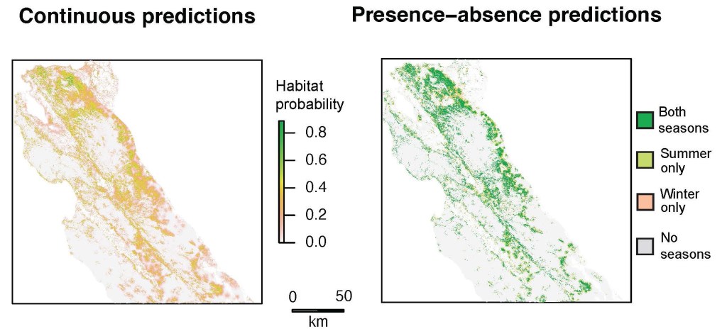
The landscape-wide predictions of habitat selection probabilities indicate significant variation in predicted suitable habitat across the study region, with the largest tracts of suitable habitat predicted throughout currently occupied tule elk range on the eastern edge of our study system (Fig. 3). There is a large gap in predicted unsuitable habitat throughout the heavily forested core area in the central Santa Cruz Mountains, surrounded by relatively suitable habitat on the coast to the southwest and in a northwest-southeast stretch of land on the inland side of the mountains. There were also some predictions of relatively suitable habitat near heavily populated areas around the San Francisco Bay (Fig. 3).

Discussion

Despite proximity to major metropolitan areas, our modeling predicted multiple large areas of suitable, but currently unoccupied, tule elk habitat in the northern Diablo Range, the inland and coastal sides of the Santa Cruz Mountains, and the northern Santa Lucia Range regions (Fig. 4). Summing the total area encompassed in the 30m habitat pixels, our model predicted 422,700–643,000 ha (1,632–2,483 mi²) of suitable habitat, depending on the season, throughout our six-county study area. Nearly one quarter of the unoccupied but suitable habitat occurred on lands already conserved.

The accuracy of the model prediction was demonstrated by its correct inclusion of currently occupied elk habitat in the northern and central Diablo Range, northern Gabilan Range east of Salinas, and the Fort Hunter Liggett population in south Monterey County. Interestingly, even modest model prediction of habitat suitability accurately included the Fort Hunter Liggett elk. Thus, the binary habitat/non-habitat map converted from the continuous probability of selection surface, though a simplification, is useful for describing tule elk habitat availability throughout the region.

The largest area of suitable but unoccupied habitat was the northern Diablo Range in Alameda and Contra Costa counties north of Interstate 580, which is roughly divided into two parallel north-south swaths. One swath runs along the East Bay foothills for 61.6 km (38.3 mi) from Crockett, California to Interstate 680 in Alameda County, and the other swath runs for 48.2 km (30.0 mi) along the higher Diablo Range elevations from Mount Diablo near Suisun Bay, south to Interstate 580 at Altamont Pass. The north-south section of Interstate 680 bisects these two parallel patches and is likely an impassable barrier for elk. The longest and next largest area of predicted but unoccupied suitable elk habitat is in the Santa Cruz Mountains in a mostly continuous 113.5 km (70.5 mi) swath of conserved lands on the inland side from Pacifica, California to the Pajaro (River) Gap. There is also a parallel but narrower swath of suitable predicted habitat in the coastal grasslands that expands in west central San Mateo County and southwestern Santa Cruz County. However, this coastal swath is not continuous, as it is divided by metropolitan Santa Cruz, California. The coastal swath runs south 86.7 km (53.9 mi) from Montara Mountain to Santa Cruz, California and then from Santa Cruz south 35.0 km (21.7 mi) along Monterey Bay to the Pajaro River mouth. The coastal lands south of the Pajaro River are considered unsuitable because we excluded areas with extensive row crop agriculture cover, as we did for urban lands elsewhere. Lastly, the model identified suitable but unoccupied tule elk habitat in the northern Santa Lucia Range, including Carmel Valley, as well as a very narrow 100 km (62.1 mi) long patch along the inland side of the Santa Lucia Range on the western side of the Salinas River Valley. This latter patch is constricted because much of the valley floor is row agriculture omitted from our model, limiting suitable elk habitat to a narrow zone between the upland shrublands, chaparral, and oak woodlands west of the valley floor, and the higher elevation coniferous forest further west.

Another key finding is the model’s prediction of lands unlikely to be utilized by tule elk. For the Santa Cruz Mountains region there are extensive conserved lands in the higher elevations populated by coast redwood and Douglas fir forest. The model correctly predicts these coniferous forests as unsuitable for tule elk. In fact, these forests are likely to act as a barrier to tule elk connectivity from the inland side to the coastal side. Therefore, we consider the northern and southern ends of the Santa Cruz Mountains as high land conservation priorities to provide important east-west linkages for future elk occupancy and demographic connectivity from the inland side of this range to the coastal grasslands further west. Similarly, the relatively open lands at the northern edge of the Santa Lucia Range constitute a high-priority east-west linkage for forest avoidant ungulates. Forest avoidance has been exhibited for decades by the large tule elk herds at Fort Hunter Liggett in Jolon, California, which was established by successful translocation in the early 1980s (Hanson and Willison 1983). Here, two herds generally utilize grasslands, oak savanna and woodlands, and chaparral, but remain confined to the inland side of the Santa Lucia Range by dense coniferous forest, despite the presence of high-quality forage a few kilometers to the west in the coastal grasslands. Forest also appears to be preventing northern range expansion for the Fort Hunter Liggett elk herds, as they have not penetrated the Los Padres National Forest to the north (James Kilber, pers. comm.).

The SLR herd resides at the southern edge of the northern Diablo Range where the habitat is relatively hotter and drier than the rest of the study area. This is a potential limitation of the model. For example, because of the steep precipitation gradient between the Diablo Range and the Pacific Ocean shore, we may have underestimated the extent of suitable habitat in the coastal grasslands. The forage most different from the SLR herd in the arid Diablo Range would be the relatively mesic coastal grasslands in western San Mateo, Santa Cruz, and Monterey counties. Unfortunately, we could not obtain input data based on radio collared elk from the coast, such as the Point Reyes herds. However, despite differences in habitat characteristics between the SLR herd and habitat in the rest of the study area with respect to aridity, forest cover, or anthropogenic development, all areas currently occupied by elk in areas intermediate between the Diablo Range and the coast were accurately predicted by the model as suitable elk habitat.

To maximize the transferability of our habitat models to novel areas, we only included habitat variables for which we could expect a direct ecological effect on tule elk, as opposed to those for which there might only be indirect or proxy effects (Melin et al. 2013), such as elevation. A possible exception to these direct effects is the puma habitat suitability layer, which was created by modeling other variables that may have resulted in some indirect influences in our modeling effort. However, this layer was the best option available to capture the direct ecological effect of predation risk on tule elk. Due to conservative modeling (no higher than second order terms) and model selection (selecting most parsimonious model as defined by AICc) to avoid overfitting the model to the SLR tule elk data, our workflow resulted in habitat inferences that should transfer well to the unoccupied areas in the west and east San Francisco Bay, and Monterey Bay regions.

Generally, the habitat responses predicted in our final model make ecological sense and conform to tule elk life history traits. There was a strong positive selection for herbaceous vegetation cover consisting of both annual and perennial forbs and grasses, which are the primary forage resources of tule elk (McCullough 1969, Mohr et al. 2022). There was an interesting avoidance of increasing shrubs until high (60%) cover, suggesting that there is perhaps either a forage intake (nutritional) or structural (thermal or hiding refuge) benefit of shrubs that only is selected for once shrub cover is high (Sawyer et al. 2007). Due to limited data at high proportions of shrub cover, we encourage caution in interpreting this selection signal. As we expected, there were important interactions between season and both tree cover and distance to water, with low tree cover selected in both seasons but with slightly more tree cover selected at a higher rate in the summer, likely due to the benefit trees provide as thermal refugia (Cook et al. 1998; Millspaugh et al. 1998).

Surprisingly, further distance to water was selected for in the summer and there was a minimal selection pattern in the winter. The opposite trend has been found for tule elk occurring in the hotter, drier Carrizo Plains (Mohr et al. 2022). This apparent lack of proximity to water makes sense when considering that our distance to waterbody variable had a strong negative response for any distance above 500 m. This suggests that standing waterbodies are more important to tule elk than stream and river sources, consistent with previous studies documenting tule elk preference for wetland habitats, consistent with their “tule” marsh namesake (McCullough 1969). Additionally, the slight positive response of tule elk to increasing distances to waterbodies at small (less than 500 m) distances suggests there is likely a forage ‘green-up’ effect at the edge of receding waterbodies that tule elk select for (Middleton et al. 2018). Tule elk’s affinity for standing waterbodies implies that the inland side of the Santa Cruz Mountains may be exceptionally suitable habitat because it is replete with reservoirs. The inland side has 13 named reservoirs, each surrounded by conserved lands from the Crystal Springs Reservoirs (San Bruno, CA, USA) in the north to Uvas Reservoir (Gilroy, CA, USA) in the south (Lanman et al. 2022a). This may be a powerful effect, as the SLR tule elk utilize steep slopes immediately surrounding San Luis Reservoir, presumably to take advantage of forage quality as the waters recede in summer and fall. This may also explain tule elk selection for increased terrain ruggedness, which was otherwise a surprising result of our model.

Although we would expect a negative response to increasing predation risk (puma habitat suitability), the relationship was nonlinear and only shifted negative at intermediate levels of predation risk, likely because pumas simultaneously select areas with prey availability. Strong avoidance responses by tule elk may only be beneficial at high risk levels when balancing other habitat needs (Cherry et al. 2017).

Finally, the slightly negative response of tule elk to roads at close distances followed expectations due to the disturbances and risks they cause, but the strong selection against increasing distance to roads at larger distances was a curious result. There are potentially some benefits associated with proximity to roads, though these would likely be proxy effects that may be better captured by other variables such as reduced predation risk (human shield effect), water availability (more roads near reservoirs/waterways), and forage (increased new plant growth in disturbed soil), or shrub cover (especially for calving) close to roads (Montgomery et al. 2013; Gavin and Komers 2006). There may be a neutral or even positive selection for proximity to minor secondary roads, while larger highways with continuous high traffic flows are actively avoided. It is important to note that while we accounted for some anthropogenic disturbance with roads, the SLR study population is not adjacent to large urban and suburban areas that are widespread in the target study region. This is a weakness of the study model as we were unable to directly model urban and/or suburban influences on tule elk habitat selection, and we thus defaulted to labeling any areas with urban development as nonhabitat. There are examples of elk utilizing human-dominated landscapes in North America, and specifically tule elk utilizing open areas inside the southeastern city limits of San Jose, California (Huntsinger et al. 1995). Future studies should gather more habitat-use data from tule elk that utilize suburban and urban-adjacent areas to investigate their selection responses.

Options for tule elk reintroduction include construction/improvement of highway over- and undercrossings. Large bridge span undercrossings (viaducts) may be the most preferred type of crossing structure by large ungulates in general (Denneboom et al. 2021). However, elk-specific data from a five-year study in Colorado found that Rocky Mountain elk utilized structural overcrossings four times more than undercrossings. When they did use undercrossings, they were found to prefer large bridge span undercrossings (viaducts) more than culverts or other types of undercrossings in the Colorado study (Kintsch et al. 2012) as well as in a meta-analysis of scientific and gray literature (Basting et al. 2022). Successful utilization of crossing structures can be predicted for mule deer (Odocoileus hemionus hemionus) and Rocky Mountain elk based on crossing structure height, width, and length (Reed and Ward 1985; Clevenger and Waltho 2005; Cramer 2012). However, paucity of California-specific and tule elk-specific data is a limitation to recommending crossing structure dimensions here. A recent publication found that all three subspecies of California elk used undercrossings below high-speed roads when an intermittent stream was present, including a tule elk herd that used culverts with openness ratios (ORs) as small as 0.3 (Lanman 2022b). However, in this study, undercrossing ORs for California elk averaged 15.0, suggesting that larger size undercrossings are preferred (Lanman 2022b). Two qualified observer records of elk attempting intermittent stream undercrossings beneath Highway 101 in Coyote Valley and near the Pajaro Gap, but a lack of conserved lands adjacent to these sites may limit passage success (Lanman et al. 2022b). Finally, design and construction of crossing structures should satisfy recommendations for multiple species (Goldfarb 2023). Importantly, a global study of wildlife overcrossing structures found that the majority in North America and Europe did not meet dimensional expert guidelines (Brennan et al. 2022).

Translocation of elk is a more rapid and less expensive reintroduction method than construction of wildlife crossing structures, based on recent California projects. For example, the Liberty Curve overcrossing at Highway 101 in Agoura Hills, California, took ten years to plan and will take three years to construct with current cost estimates at $90 million. The Laurel Curve undercrossing at Highway 17 cost $23.5 million and ten years to plan and complete. A smaller undercrossing structure at Trout Creek under Highway 17 is estimated to cost $11.2 million but may lack adequate size and other desirable characteristics for elk to select for use (Lanman et al. 2022b). These costs are conservative as they do not include the cost of land acquisitions on both sides of undercrossings, which are exceptionally high in the study area. However, translocation may pose unique risks versus natural range expansion in two scenarios. First, capture and relocation of wildlife yields significant risks to individual animal welfare and can result in unwanted outcomes, including mortality (Arnemo et al. 2006). Translocated elk are stressed by their capture, captivity, quarantine, and ultimate release into novel environments, with measurable physiological effects that last as long as six weeks (Pero et al. 2022). Second, translocations into regions with habitat of heterogeneous quality or that is not contiguous may be unsuccessful or become wholly reliant on continued follow up releases to maintain a viable population (Smith et al. 2023). However, well planned conservation-based translocations have consistently yielded intended benefits without unintended harms and are part of planned recovery actions for 70% of listed threatened and endangered taxa in the United States (Novak et al. 2021).

Although translocations of elk to unoccupied regions may be relatively cost effective and expedient, translocations without connectivity would fail to alleviate the inbreeding depression that threatens this already genetically depauperate subspecies (Sacks et al. 2016). Translocations enable elk to bypass highway infrastructure, but once herds are re-established, highways and other infrastructure would still present continued barriers to gene flow, as well as risks from elk-vehicle collisions, as illustrated by the 16 recently recorded elk-vehicle collisions on Highway 152 (Pacheco Pass Highway) bordering San Luis Reservoir.

For wildlife linkages from the Santa Cruz Mountains region to the Diablo and Gabilan Ranges, Highway 101 is the critical barrier for bidirectional long-term gene flow (Lanman et al. 2022b). Highway 101 is also the barrier to westward range expansion for elk from the Gabilan Range to the inland and northern portions of the Santa Lucia Range in Monterey County. The tule elk herds at Fort Hunter Liggett appear to be confined from northward range expansion to north Monterey County by the Los Padres National Forest, leaving highway crossing(s) across Highway 101 as the only solution for long-term connectivity to the Gabilan Range. However, significant row crop agriculture along Highway 101 in the Salinas Valley may make locating a freeway overcrossing in northern Monterey County difficult. In the northern Diablo Range Interstates 580 and 680 present barriers to connectivity of southern Alameda County tule elk to the East Bay Foothills and further north in the Diablo Range. Here, undercrossings might be improved by land conservation on both sides of the Interstate 680 undercrossing at Alameda Creek, and of Interstate 580 near Altamont Pass. Urban and suburban development from Dublin to Martinez along the Interstate 680 corridor is an additional barrier to connectivity between the East Bay Foothills and the northern Diablo Range proper, requiring careful study if linkages between the two ranges north of Interstate 580 are feasible. Interestingly, it is possible that the Grizzly Island tule elk herd in Suisun Bay might eventually expand into Contra Costa County, as occurred in 2006 when a bull elk that was relocated to Grizzly Island was tracked swimming across Suisun Bay to Contra Costa County, a straight-line distance of almost 4 km (J. Hobbs, CDFW, pers. comm.; Moyle et al. 2014). Multiple crossings by large elk herds from Mare Island south across the Carquinez Strait were described historically (Davis and Watson 1929).

Both translocation and natural range expansion via highway over- and undercrossings restore elk to new locations, posing similar risks of conflict (e.g. fence damage, elk-vehicle collisions, crop depredation), disease transmission, and competition with domestic and native grazers for forage (Schroeder and Stewart 2022). Both approaches will require public education regarding management of human-wildlife conflict related to property and crop damage, non-competitive conflict with domestic animals, competition with domestic livestock, and habituation to humans as essential elements for success. Human-elk conflict issues should be reported using the CDFW Wildlife Incident Reportingsystem allowing CDFW to manage issues using established protocols (Denryter and Heeren 2021).

In addition to the potential ecological benefits of restoring a native ungulate grazer to the grassland, shrubland, and oak woodland habitats in these regions (Lanman et al. 2022a), there are substantial societal benefits to be gained from the return of tule elk to areas near large populations. As demonstrated in multiple studies of pyric herbivory, namely the combination of prescribed or cultural burns and large mammal herbivory, the primary benefit of elk restoration to these increasingly wildfire-prone coastal regions may be reduction of understory fire fuel loads which enable crown fires in oak woodlands (Lecomte et al. 2019; Defrees et al. 2020). Ironically, the many decades of land conservation in the Study Area have likely increased wildfire risk, due to wildfire suppression and diminished cattle grazing, a phenomenon similar to the increased in wildfires secondary to farm abandonment in southern Europe. These trends can be mitigated by the introduction of wild large herbivores such as elk (Rouet-Leduc et al. 2021). Wildlife viewing and hunting opportunities, including indigenous hunting, will accrue once tule elk populations become sustained. These activities are associated with sizeable economic implications. The U.S. Fish and Wildlife Service’s 2011 survey of fishing, hunting, and wildlife-associated recreation in California documented that public non-consumptive appreciation of wildlife led to $3.8 billion in expenditures, in addition to $964 million of spending by hunters (USFWS 2012). Despite these potential benefits, the restoration of tule elk to this area comes with significant challenges. While unoccupied suitable tule elk habitat may exist, incompatible land uses, including potential conflicts with ranchers over competition for grazing habitat and fence damages (Hanbury-Brown et al. 2021), conflicts with farmers over crop depredation (Vercauteren et al. 2005), and potential vehicle collisions on roads (Schwartz et al. 2020;  Sevigny et al. 2021), have made securing suitable release sites a major challenge facing resource managers for several decades (BLM 1992). We recommend restoration efforts be carefully considered and managed (Huber et al. 2014; Denryter and Heeren 2021), including consideration of social tolerance of land owners adjacent to release sites and future means to control populations (i.e., regulated harvest, translocation, etc.) that are consistent with management goals and objectives (CDFW 2018). Whether tule elk populations are restored through human-mediated translocations, habitat and highway infrastructure connectivity enhancement, or a combination of approaches is a question for wildlife and land managers to address via engagement of multiple stakeholders in a constitutive planning process (Clark and Vernon 2017).

In sum, the results herein suggest the existence of multiple patches of habitat suitable for tule elk that are presently unoccupied, and which lie within their former historical range throughout Alameda, Contra Costa, San Mateo, Santa Clara, Santa Cruz, and Monterey counties. Despite their proximity to major urban areas, 122 years of land conservation has resulted in relatively high percentages of protected lands in the study area (Yaryan and Verardo 2000; Lanman 2022a). These predicted habitat patches are generally contiguous, although fragmented by major federal highways and at least two other major barriers to natural range expansion: the city of Santa Cruz in the coastal grasslands, and dense forest in the Santa Cruz Mountains and Santa Lucia Range. Ground truthing will be required before management recommendations can be made, as the long swaths of land identified by this analysis may have fine but significant barriers to contiguity not assessable by the model, and the habitat predictions themselves may need validation given the novel, unoccupied area in which they were predicted.

Acknowledgments

The authors thank Jim Kilber, fish and wildlife biologist for Fort Hunter Liggett, for his up-to-date observations of the tule elk herds in southern Monterey County, as well as the California Department of Fish and Wildlife teams who, over more than a century, have carefully restored this nearly extirpated endemic California elk subspecies.

Literature Cited

• AECOM. 2021. Monterey County Regional Conservation Investment Strategy. Oakland, CA, USA. Prepared for the Transportation Agency for Monterey County, Salinas, CA, USA. Available from: https://www.tamcmonterey.org/files/ed9205e45/MontereyCountyRCIS_Final_Jun2021.pdf
• Akaike, H. 1974. Stochastic theory of minimal realization. IEEE Transactions on Automatic Control. AC19(6):667–674. http://www.doi.org/10.1109/TAC.1974.1100707
• Allouche, O., A. Tsoar, and R. Kadmon. 2006. Assessing the accuracy of species distribution models: prevalence, kappa and the true skill statistic (tss). Journal of Applied Ecology 43(6):1223–1232. https://doi.org/10.1111/j.1365-2664.2006.01214.x
• Allred, B. W., B. T. Bestelmeyer, C. S. Boyd, C. Brown, K. W. Davies, M. C. Duniway, L. M. Ellsworth, T. A. Erickson, S. D. Fuhlendorf, T. V. Griffiths, V. Jansen, M. O. Jones, J. Karl, A. Knight, J. D. Maestas, J. J. Maynard, S. E. McCord, D. E. Naugle, H. D. Starns, D. Twidwell, and D. R. Uden. 2021. Improving landsat predictions of rangeland fractional cover with multitask learning and uncertainty. Methods in Ecology and Evolution 12(5):841–849. https://doi.org/10.1111/2041-210X.13564
• Arnemo, J. M., P. Ahlqvist, R. Andersen, F. Berntsen, G. Ericsson, J. Odden, S. Brunberg, P. Segerström, and J. E. Swenson. 2006. Risk of capture-related mortality in large free-ranging mammals: experiences from Scandinavia. Wildlife Biology. 12(1):109–113. http://www.doi.org/10.2981/0909-6396(2006)12[109:ROCMIL]2.0.CO;2
• Basting, P., K. Bishton, K. Brown, T. Smithson, and G. Woolley. 2022. A literature analysis to determine optimal wildlife crossing structure size. Colorado Department of Transportation, Denver, CO, USA. Available from: https://www.codot.gov/programs/research/pdfs/2022/2022-01
• Batter, T. J., J. P. Bush, and B. N. Sacks. 2021. Assessing genetic diversity and connectivity in a tule elk (Cervus canadensis nannodes) metapopulation in Northern California. Conservation Genetics 22(6):889–901. https://www.doi.org/10.1007/s10592-021-01371-0
• Bay Area Open Space Council (BAOSC). 2019. The Conservation Lands Network 2.0 Report. Berkeley, CA, USA. Available from: https://www.bayarealands.org/maps-data/
• Boyce, M. S., P. R. Vernier, S. E. Nielsen, and F. K. A. Schmiegelow. 2002. Evaluating resource selection functions. Ecological Modelling 157:281–300. https://doi.org/10.1016/S0304-3800(02)00200-4
• Brennan, L., E. Chow, and C. Lamb. 2022. Wildlife overpass structure size, distribution, effectiveness, and adherence to expert design recommendations. PeerJ 10:e14371. http://www.doi.org/10.7717/peerj.14371
• Burcham, L. T. 1957. California range land: an historico-ecological study of the range resources of California. Department of Natural Resources, Division of Forestry, Sacramento, CA, USA.
• Bureau of Land Management (BLM). 1992. Tenth report to congress: the tule elk in California. Department of the Interior, Bureau of Land Management, Sacramento, CA, USA.
• Calenge, C. 2006. The package “adehabitat” for the R software: a tool for the analysis of space and habitat use by animals. Ecological Modelling 197:516–519. https://doi.org/10.1016/j.ecolmodel.2006.03.017
• California Department of Fish and Wildlife (CDFW). 2018. Elk Conservation and Management Plan. California Department of Fisheries and Wildlife, Sacramento, CA, USA. Available from: https://nrm.dfg.ca.gov/FileHandler.ashx?DocumentID=162912&inline
• California Protected Areas Database (CPAD). 2023. GreenInfo Network, Oakland, CA, USA. Available from: https://www.calands.org/cpad/
• Cherry, M. J., R. J. Warren, and L. M. Conner. 2017. Fire-mediated foraging tradeoffs in white-tailed deer. Ecosphere 8(4). https://doi.org/10.1002/ecs2.1784
• Clark, S. G., and M. E. Vernon. 2017. Elk management and policy in southern Greater Yellowstone: assessing the constitutive process. Policy Science 50(2):295–316. http://www.doi.org/10.1007/s11077-016-9268-7
• Clevenger, A. P., and N. Waltho. 2005. Performance indices to identify attributes of highway crossing structures facilitating movement of large mammals. Biological Conservation 121:453–464. https://doi.org/10.1016/j.biocon.2004.04.025
• Cobb, M. A. 2010. Spatial ecology and population dynamics of tule elk (Cervus elaphus nannodes) at Point Reyes National Seashore, California. Dissertation, University of California, Berkeley, CA, USA. Available from:https://escholarship.org/uc/item/2wt3h3rc
• Cook, J. G., L. L. Irwin, L. D. Bryant, R. A. Riggs, and J. W. Thomas. 1998. Relations of forest cover and condition of elk: a test of the thermal cover hypothesis in summer and winter. Wildlife Monographs 141:3–61.
• Cramer, P. 2012. Determining wildlife use of crossing structures under different scenarios. Utah Department of Transportation, Taylorsville, UT, USA. Available from: https://rosap.ntl.bts.gov/view/dot/24501   
• Dasmann, W. P. 1975. Big game of California. California Fish and Game, Sacramento, CA, USA.
• Davis, W. H., and D. S. Watson. 1929. Seventy-Five Years in California: A History of Events and Life in California: Personal, Political and Military. J. Howell, Berkeley, CA, USA.
• Defrees, D., J. P. Averett, M. J. Wisdom, and B. A. Endress. 2020. Interactive effects of fuels reduction and large herbivores on shrub assemblages in dry conifer forests of the interior west, USA. Forest Ecology and Management 463:118031. https://doi.org/10.1016/j.foreco.2020.118031
• Dellinger, J. A., B. Cristescu, J. Ewanyk, D. J. Gammons, D. Garcelon, P. Johnston, Q. Martins, C. Thompson, T. W. Vickers, C. C. Wilmers, H. U. Wittmer, and S. G. Torres. 2020. Using mountain lion habitat selection in management. Journal of Wildlife Management 84:359–371. https://doi.org/10.1002/jwmg.21798
• Denneboom, D., A. Bar-Massada, and A. Shwartz. 2021. Factors affecting usage of crossing structures by wildlife: a systematic review and meta-analysis. Science of The Total Environment. 777:146061. https://doi.org/10.1016/j.scitotenv.2021.146061
• Denryter, K., and A. Heeren. 2021. Thematic and hotspot analysis of human-elk conflicts statewide in California. California Fish and Wildlife Journal, Human-Wildlife Interactions Special Issue 107(3). https://doi.org/10.51492/cfwj.hwisi.4
• Denryter, K., and J. K. Fischer. 2022. Mitigating anthropogenic barriers to facilitate distributional shifts helps reduce vulnerability of a large herbivore to climate change. Animal Conservation 25(5):718–731. https://www.doi.org/10.1111/acv.12776
• Dewitz, J., and U.S. Geological Survey (USGS). 2021. National Land Cover Database (NLCD) 2019 Products (version 2.0, June 2021). U.S. Geological Survey data release. Available from: doi:10.5066/P9KZCM54
• Duncan, K. E. 1988. Computer assisted home range analysis of tule elk in the Diablo range of California. Thesis, San Jose State University, San Jose, CA, USA. Available from: https://scholarworks.sjsu.edu/cgi/viewcontent.cgi?article=4060&context=etd_theses
• Eastwood, A. 1897. The coniferae of the Santa Lucia Mountains. Erythea 5:71–74.
• Evermann, B. W. 1915. An attempt to save California elk. California Fish and Game 1:85–95.
• Fry, W. 1924. The California grizzly. Sequoia National Park, Historic Series, Nature Guide Service Bulletin 2:4.
• Gavin, S. D., and P. E. Komers. 2006. Do pronghorn (Antilocapra americana) perceive roads as a predation risk? Canadian Journal of Zoology 84:1775–1780. https://www.doi.org/10.1139/Z06-175
• Gesch, D., M. Oimoen, S. Greenlee, C. Nelson, M. Steuck, and D. Tyler. 2002. The national elevation dataset. Photogrammetric Engineering and Remote Sensing 681:5–32.
• Goldfarb, B. 2023. Crossings: How Road Ecology is Shaping the Future of Our Planet. First edition. W.W. Norton & Company, New York, NY, USA.
• Gorelick, N., M. Hancher, M. Dixon, S. Ilyushchenko, D. Thau, and R. Moore. 2017. Google Earth Engine: Planetary-scale geospatial analysis for everyone. Remote Sensing of Environment 202:18–27. https://doi.org/10.1016/j.rse.2017.06.031
• Goss, M., D. L. Swain, J. T. Abatzoglou, A. Sarhadi, C. A. Kolden, A. P. Williams, and N. S. Diffenbaugh. 2020. Climate change is increasing the likelihood of extreme autumn wildfire conditions across California. Environmental Research Letters. 15(9):094016. https://www.doi.org/10.1088/1748-9326/ab83a7
• Grinnell, J. 1933. Review of the recent mammal fauna of California. University of California Publications in Zoology 40(2):71–224.
• Hall Defrees, D., J. P. Averett, M. J. Wisdom, and B. A. Endress. 2020. Interactive effects of fuels reduction and large herbivores on shrub assemblages in dry conifer forests of the interior west, USA. Forest Ecology and Management 463:118031. https://doi.org/10.1016/j.foreco.2020.118031
• Hanbury-Brown, A. R., J. W. Stackhouse, and L. T. Macaulay. 2021. Elk conflict with beef and dairy producers poses wildlife management challenges in northern California. Ecology and Society 26(1):23. https://doi.org/10.5751/ES-12283-260123
• Hanson, M. T., and J. M. Willison. 1983. The 1978 relocation of tule elk at Fort Hunter Liggett—reasons for its failure. Cal-Neva Wildlife Transactions 19.2:43–49. Available from: https://www.wildlifeprofessional.org/western/transactions/transactions_1983_5.pdf
• Hijmans, R. 2020. ‘raster’: Geographic Data Analysis and Modeling. R package. Available from: https://CRAN.R-project.org/package=raster Accessed 20 Dec 2022.
• Hirzel, A. H., G. Le Lay, V. Helfer, C. Randin, and A. Guisan. 2006. Evaluating the ability of habitat suitability models to predict species presences. Ecological Modelling 199(2):142–152. https://doi.org/10.1016/j.ecolmodel.2006.05.017
• Hopkins, R. A. 1989. Ecology of the puma in the Diablo Range, California. Dissertation, University of California, Berkeley, CA, USA.
• Huber, P. R., S. E. Greco, N. H. Schumaker, and J. Hobbs. 2014. A priori assessment of reintroduction strategies for a native ungulate: using hexsim to guide release site selection. Landscape Ecology 29(4):689–701. https://doi.org/10.1007/s10980-014-0006-2
• Huntsinger, L., J. Fried, and L. Buttolph. 1995. The elk, the cow, the ranger, and the rolex: urban wildland resource management conflict at Mt Diablo State Park, California. Natural Resources and Environmental Issues 3:art14. Available from: https://digitalcommons.usu.edu/nrei/vol3/iss1/14
• Johnson, D. H. 1980. The comparison of usage and availability measurements for evaluating resource preference. Ecology 61:65–71. https://doi.org/10.2307/1937156
• Jones, M. O., B. W. Allred, D. E. Naugle, J. D. Maestas, P. Donnelly, L. J. Metz, J. Karl, R. Smith, B. Bestelmeyer, C. Boyd, J. D. Kerby, and J. D. McIver. 2018. Innovation in rangeland monitoring: annual, 30 m, plant functional type percent cover maps for U.S. rangelands, 1984–2017. Ecosphere 9(9). https://doi.org/10.1002/ecs2.2430
• Kintsch, J., P. Cramer, P. Singer, and M. Cowardin. 2021. State Highway 9 Wildlife Mitigation Monitoring. Report CDOT-2021-01. Colorado Department of Transportation, Applied Research and Innovation Branch, Denver, CO, USA.
• Lanman, R. B., W.C. Leikam, M. V. Arellano, A. Leventhal, V. Lopez, R. A. Phillips, J. A. Phillips, and K. Denryter. 2022a. A review of considerations for restoration of tule elk to the San Francisco Peninsula and northern Monterey Bay counties of California. California Fish and Wildlife Journal 108:62–93. https://www.doi.org/10.51492/cfwj.108.14
• Lanman, R. B., J. Kilber, J. Cann, H. Carrington, E. Zulliger, J. Bush, F. W. Weckerley, and T. J. Batter. 2022b. Road and highway undercrossings as potential critical linkages for California’s elk populations. California Fish and Wildlife Journal 108:158–169. https://www.doi.org/10.51492/cfwj.108.18
• Lecomte, X., M. C. Caldeira, F. X. Catry, P. M. Fernandes, R. B. Jackson, and M. N. Bugalho. 2019. Ungulates mediate trade‐offs between carbon storage and wildfire hazard in Mediterranean oak woodlands. Journal of Applied Ecology 56(3):699–710. http://doi.org/10.1111/1365-2664.13310
• Lehman, C. P., C. T. Rota, J. D. Raithel, and J. J. Millspaugh. 2018. Pumas affect elk dynamics in absence of other large carnivores: Pumas Alone Suppress Elk Population Growth. Journal of Wildlife Management 82(2):344–353. https://www.doi.org/10.1002/jwmg.21392
• McCorriston, J. 1994. Acorn eating and agricultural origins: California ethnographies as analogies for the ancient Near East. Antiquity 68:97–107. https://doi.org/10.1017/S0003598X00046238
• McCullough, D. R. 1969. The tule elk, its history, behavior, and ecology. University of California Publications in Zoology 88:1–209.
• McCullough, D., J. Fischer, and J. Ballou. 1996. From bottleneck to metapopulation: recovery of the tule elk in California. Pages 377–378 in D. R. McCullough, editor. Metapopulations and Wildlife Conservation. Second edition. Island Press, Washington, D.C., USA.
• Melin, M., P. Packalen, J. Matala, L. Mehtatalo, and J. Pusenius. 2013. Assessing and modeling moose (Alces alces) habitats with airborne laser scanning data. International Journal of Applied Earth Observation and Geoinformation 23:389–396. https://doi.org/10.1016/j.jag.2012.11.004
• Meredith, E. P., J. A. Rodzen, J. D. Banks, R. Schaefer, H. B. Ernest, T. R. Famula, and B. P. May. 2007. Microsatellite analysis of three subspecies of elk (Cervus elaphus) in California. Journal of Mammalogy 88:801–808. https://doi.org/10.1644/06-MAMM-A-014R.1
• Middleton, A. D., J. A. Merkle, D. E. McWhirter, J. G. Cook, R. C. Cook, P. J. White, and M. J. Kauffman. 2018. Green-wave surfing increases fat gain in a migratory ungulate. Oikos 127(7):1060–1068. https://doi.org/10.1111/oik.05227
• Millspaugh, J. J., K. J. Raedeke, G. C. Brundige, and C. C. Willmott. 1998. Summer bed sites of elk (Cervus elaphus) in the Black Hills, South Dakota: considerations for thermal cover management. American Midland Naturalist 139(1):133–140. https://doi.org/10.1674/0003-0031(1998)139[0133:SBSOEC]2.0.CO;2
• Mohr, A. S., R. Stafford, and W. T. Bean. 2022. Tule elk selection of surface water and forage is mediated by season and drought. California Fish and Wildlife Journal, Proceedings of the 14th Biennial Deer and Elk Workshop 108(3). http://www.doi.org/10.51492/cfwj.108.19
• Montgomery, R. A., G. J. Roloff, and J. J. Millspaugh. 2013. Variation in elk response to roads by season, sex, and road type. Journal of Wildlife Management 77:313–325. https://doi.org/10.1002/jwmg.462
• Moyle, P., A. D. Manfree, and P. L. Fiedler. 2014. Suisun Marsh, Ecological History and Possible Futures. University of California Press, Berkeley, CA, USA.
• Murtaugh, P. A., 2009. Performance of several variable‐selection methods applied to real ecological data. Ecology Letters, 12:1061–1068. https://doi.org/10.1111/j.1461-0248.2009.01361.x
• Novak, B. J., R. Phelan, and M. Weber. 2021. U.S. conservation translocations: over a century of intended consequences. Conservation Science and Practice 3(4):csp2.394. https://doi.org/10.1111/csp2.394
• Northrup, J. M., M. B. Hooten, C. R. Anderson, and G. Wittemyer. 2013. Practical guidance on characterizing availability in resource selection functions under a use-availability design. Ecology 94:1456–1463. https://doi.org/10.1890/12-1688.1
• Pero, E. M., M. C. Chitwood, A. M. Hildreth, B. J. Keller, R. J. Millspaugh, J. A. Sumners, L .P. Hansen, J. L. Isabelle, C. W. Breuner, and J. J. Millspaugh. 2022. Physiological acclimation of elk during population restoration in the Missouri Ozarks, USA. Conservation Physiology 10(1):coac009. https://doi.org/10/1093/conphys/coac009 
• Phillips, J. A. 1985. Acclimation of reintroduced tule elk in the Diablo Range, California. Thesis, San Jose State University, San Jose, CA, USA.
• Phillips, J. A. 2023. A citizen’s guide to the tule elk of California. Nature Based Teaching, Santa Cruz, CA. Available from: https://naturebasedteaching.com/tule-elk-pr17/
• Potter, C., and O. Alexander. 2022. Machine learning to understand patterns of burn severity from the SCU Lightning Complex Fires of August 2020. California Fish and Wildlife Journal. 108:108–120. https://www.doi.org/10.51492/cfwj.108.6 
• Reed, D. F., and A. L. Ward. 1985. Efficacy of methods advocated to reduce deer-vehicle accidents: research and rationale in the USA. Routes et faune sauvage. Service d’Etudes Techniques de Routes et Autoroutes, Bagneaux, France.
• Rouet‐Leduc, J., Pe’er, G., Moreira, F., Bonn, A., Helmer, W., Shahsavan Zadeh, S. A. A., Zizka, A,, and F. Van Der Plas. 2021. Effects of large herbivores on fire regimes and wildfire mitigation. Journal of Applied Ecology 58(12):2690–2702. https://doi.org/10.1111/1365-2664.13972
• Sacks, B. N., Z. T. Lounsberry, T. Kalani T, E. P. Meredith, and C. Langner. 2016. Development and characterization of 15 polymorphic dinucleotide microsatellite markers for tule elk using HiSeq3000. Journal of Heredity 107(7):666–669. https://doi.org/10.1007/s12686-020-01184-2
• Sawyer, H., R. M. Nielson, F. G. Lindzey, L. Keith, J. H. Powell, and A. A. Abraham. 2007. Habitat selection of rocky mountain elk in a nonforested environment. Journal of Wildlife Management 71:868–874. https://doi.org/10.2193/2006-131
• Schroeder, C., and K. Stewart. 2022. Unintended consequences of species translocations: changes in distribution and habitat selection of mule deer following introduction of elk. California Fish and Wildlife Journal, Proceedings of the 14th Biennial Deer and Elk Workshop 108(3). http://www.doi.org/10.51492/cfwj.108.16
• Schwartz, A. L. W., F. M. Shilling, and S. E. Perkins. 2020. The value of monitoring wildlife roadkill. European Journal of Wildlife Research 66(1):18. https://doi.org/10.1007/s10344-019-1357-4
• Sevigny, J., A. Summers, G. Kalisz, and K. McAllister. 2021. Identification of elk-vehicle incident hotspots on State Route 20 in Washington State. Landscape Ecology 36(6):1685–1698. https://doi.org/10.1007/s10980-021-01238-2
• Sharsmith, H. K. 1945. Flora of the Mount Hamilton Range of California (a taxonomic study and floristic analysis of the vascular plants). American Midland Naturalist 34(2):289–367.
• Smith, J. B., D. A. Keiter, S. J. Sweeney, R. S. Miller, P. E. Schlichting, and J. C. Beasley. 2023. Habitat quality influences trade-offs in animal movement along the exploration–exploitation continuum. Scientific Reports 13(1):4814. https://doi.org/10.1038/s41598-023-31457-3
• Stephens, S. L., and D. L. Fry. 2005. Fire history in coast redwood stands in the northeastern Santa Cruz Mountains, California. Fire Ecology 1(1):2–19. https://doi.org/10.4996/fireecology.0101002
• Thomas, J. H. 1975. Flora of the Santa Cruz Mountains of California: A Manual of the Vascular Plants. Stanford University Press, Stanford, CA, USA.
• Thompson, K. 1961. Riparian forests of the Sacramento Valley, California. Annals of the Association of American Geographers 51(3): 294–315. https://doi.org/10.1111/j.1467-8306.1961.tb00380.x
• Toweill, D. E., J. W. Thomas, and R. E. McCabe. 2002. North American Elk: Ecology and Management. First. Smithsonian Institution, Washington, D.C., USA.
• U.S. Census Bureau (USCB). 2019. TIGER/Line Shapefiles (machinereadable data files). Available from: https://www2.census.gov/geo/pdfs/maps-data/data/tiger/tgrshp2019/TGRSHP2019_TechDoc.pdf
• U.S. Fish and Wildlife Service (USFWS). 2012. 2011 National survey of fishing, hunting, and wildlife-associated recreation state overview. U.S. Fish and Wildlife Service, Washington, D.C, USA. Available from: https://digitalmedia.fws.gov/digital/collection/document/id/858/
• Van Dyke, T. S. 1902. The deer and elk of the Pacific coast. Pages 167–256 in T. S. Roosevelt, T. S. Van Dyke, D. G. Elliott, and A. J. Stone, editors.The Deer Family. MacMillan, New York, NY, USA.
• Venables, W. N., and B. D. Ripley. 2002. Modern Applied Statistics with S. Springer, New York, NY, USA.
• Vercauteren, K. C., N. W. Seward, D. L. Hirchert, M. L. Jones, and S. F. Beckerman. 2005. Dogs for reducing wildlife damage to organic crops: a case study. Pages 286–293 in Proceedings of the 11th Wildlife Damage Management Conference. National Wildlife Research Center, Fort Collins, CO, USA.
• Watt, L. A. 2015. The continuously managed wild: tule elk at Point Reyes National Seashore. Journal of International Wildlife Law & Policy 18(4):289–308. https://doi.org/10.1080/13880292.2015.1096159
• Williams, C. L., B. Lundrigan, and O. E. Rhodes. 2004. Microsatellite DNA variation in tule elk. Journal of Wildlife Management 68:109–119. https://doi.org/10.2193/0022-541X(2004)068[0109:MDVITE]2.0.CO;2
• Wisdom, M. J., H. K. Preisler, L. M. Naylor, R. G. Anthony, B. K. Johnson, and M. M. Rowland. 2018. Elk responses to trail-based recreation on public forests. Forest Ecology and Management 411:223–233. https://doi.org/10.1016/j.foreco.2018.01.032
• Yaryan, W., and D. Verardo. 2000. The Sempervirens Story: A Century of Preserving California’s Ancient Redwood Forest, 1900–2000. Sempervirens Fund, Los Altos, CA, USA.