Experimental gillnet study to inform future large fish monitoring in the San Francisco Estuary

FULL RESEARCH ARTICLE

Dylan Keating Stompe^1,2* and James A. Hobbs³

¹ California Department of Fish and Wildlife, Bay Delta Region, 2825 Cordelia Road, Unit 100, Fairfield, CA 94534, USA (former)
² California Department of Fish and Wildlife, Marine Region, 1010 Riverside Parkway, West Sacramento, CA 95605, USA (current)
https://orcid.org/0000-0002-5994-2014
³ California Department of Fish and Wildlife, Bay Delta Region, 2109 Arch Airport Road, Stockton, CA 95206, USA
  https://orcid.org/0000-0002-4052-9000

*Corresponding Author: dylan.stompe@wildlife.ca.gov

Published 27 December 2024 • doi.org/10.51492/cfwj.110.16

Abstract

Fishery independent monitoring in the San Francisco Estuary (SFE) includes extensive coverage by the many trawl- and seine-based surveys of the Interagency Ecological Program (IEP). These surveys primarily sample small forage fishes and/or juvenile life stages of larger fishes due to the relatively small net dimensions, mesh sizes, and tow speeds. As a result, the adult life stage of many SFE fish species is not completely sampled, representing a shortcoming in our ability to track changes in age-structured regional fish assemblages. To help fill this monitoring gap, we conducted an experimental gillnetting effort in the spring of 2023. We employed American Fisheries Society experimental gillnets in a stratified random sampling design in the North Delta, California, USA. In total, we caught 16 fish species during 141 approximately one-hour gillnet sets, including 33 paired day and night sets to test diurnal effects on catch. On average, fishes caught in this study were substantially larger than those caught by trawl- and seine-based surveys. Ordination analyses revealed a high degree of overlap in sampled fish assemblages between the three North Delta subregions (Cache Slough Complex, Lindsey Slough Complex, Liberty Slough Complex), with significant differences detected for only the Lindsey Slough Complex. When testing diel effects on catch, significant differences in species assemblage were seen between day and night sets. However, differences in catch may not justify the added risk and complexities of night sampling except for targeted studies of benthic predators (catfishes). Finally, while over 3,000 PIT tags were deployed (primarily in Striped Bass) between this and another nearby study, only 6 PIT tags were recovered, demonstrating that greater effort or different methodologies would be required to generate mark-recapture abundance estimates in this open and highly dynamic system. This study demonstrates the efficacy of experimental gillnets in sampling the large fish community within portions of the SFE and may inform future SFE large fish monitoring.

Key words: Delta, gillnet, Interagency Ecological Program, large fish, monitoring, San Francisco Estuary

Citation: Stompe, D. K., and J. A. Hobbs. 2024. Experimental gillnet study to inform future large fish monitoring in the San Francisco Estuary. California Fish and Wildlife Journal 110:e16.

Editor: Travis Apgar, Water Branch

Submitted: 22 February 2024; Accepted: 9 August 2024

Copyright: ©2024, Stompe and Hobbs. This is an open access article and is considered public domain. Users have the right to read, download, copy, distribute, print, search, or link to the full texts of articles in this journal, crawl them for indexing, pass them as data to software, or use them for any other lawful purpose, provided the authors and the California Department of Fish and Wildlife are acknowledged.

Funding: This study was funded by the Department of Water Resources as part of the Interagency Ecological Program.

Competing Interests: authors have not declared any competing interests.

Introduction

The San Francisco Estuary (SFE) is a dynamic and highly modified environment consisting of two primary river inputs, an inverted, mostly freshwater delta (Delta), and a series of progressively more saline bays that terminate at the Pacific Ocean (Conomos et al. 1985). Freshwater inputs are impounded to store water and regulate river flow, while the Delta is highly channelized and largely disconnected from its historic marshplain and floodplain habitats. Two major water export facilities, the Central Valley Project (CVP) and the State Water Project (SWP), operate in the southern portion of the Delta, diverting a substantial portion of the freshwater inflow for agricultural and municipal use (Lund et al. 2007). The SFE is also a highly invaded ecosystem, hosting a suite of non-native invertebrates, vegetation, and fish species (Cohen and Carlton 1998). Consequently, some introduced and many native fishes have experienced declines in abundance (e.g., Striped Bass, Morone saxatilis; Stevens et al. 1985), extirpation (Sacramento Perch, Archoplites interruptus; Crain and Moyle 2011), or even extinction (Thicktail Chub, Gila crassicauda; Moyle 2002).

To track the effects of water infrastructure on sensitive fish populations and the general fish assemblage, long-term monitoring surveys were established by various public agencies and university groups, collectively forming the Interagency Ecological Program (IEP; Tempel et al. 2021). The monitoring programs of the IEP are implemented by the California Department of Fish and Wildlife (CDFW), the U.S. Fish and Wildlife Service (USFWS), the California Department of Water Resources (CDWR), the U.S. Geological Survey (USGS), and the University of California, Davis (UCD). These studies have been used to identify long-term declines in fish abundance (Sommer et al. 2007), habitat use (Sommer et al. 2011), and subregional distribution (Stompe et al. 2022) within the SFE but have largely focused on small fish species or the juvenile life stages of large-bodied fishes. A multitude of short-term special studies, some of which have focused on large-bodied fishes, have been conducted by members of the IEP and other research and consulting entities. However, their short time scale limits their utility in identifying long-term trends or responses to systemic changes in water management.

Most of the current long-term fish surveys in the SFE employ trawl-based gear types designed to capture small, pelagic forage fishes (< 92 mm, 95th percentile (2019); CDFW Fall Midwater Trawl, CDFW Summer Townet Survey, USFWS Enhanced Delta Smelt Monitoring, etc.), while others use gear better suited to capture small littoral fishes (< 118 mm, 95th percentile (2019); USFWS Beach Seine Survey), small to large littoral fishes (< 330 mm, 95th percentile (2019); USFWS Delta Boat Electrofishing Survey; McKenzie and Mahardja 2021; McKenzie et al. 2022), and small to medium benthic fishes (< 235 mm, 95th percentile (2019); UCD Otter Trawl, CDFW Bay Study Otter Trawl; Honey et al. 2004). Of these surveys, only the USFWS Delta Boat Electrofishing Survey regularly catches large fishes. However, it is limited to sampling shallow freshwater habitats, precluding its ability to fully capture large fish assemblages in pelagic, benthic, and saline environments (Warry et al. 2013). The other gear types primarily select for small fishes due to the relatively slow travel speed, small net dimension, and small mesh sizes, making these surveys less efficient as fish increase in size and can more effectively avoid and escape capture (Klein et al. 2019). Other long-term studies of large-bodied fishes (CDFW Striped Bass Study, CDFW Adult Sturgeon Study) were useful for tracking trends in the abundance and demographics of target species but were limited both spatially and in their utility for non-target species and are no longer funded as part of IEP monitoring. As a result, large fishes and the adult life stage of many fishes are under-sampled by most IEP surveys, representing a gap in SFE fish assemblage monitoring.

Large fishes carry high recreational value (e.g., Largemouth Bass [Micropterus salmoides]) and cultural value (e.g., Sacramento Sucker [Catostomus occidentalis], Sacramento Splittail [Pogonichthys macrolepidotus], and Green Sturgeon [Acipenser medirostris]) and represent the spawning stock for many of the smaller fishes sampled in most IEP monitoring programs. Additionally, large fishes such as Striped Bass and Sacramento Pikeminnow (Ptychocheilus grandis) are high order piscivores (Moyle 2002) that have the potential to drive prey species behavior and abundance (Nobriga and Smith 2020; Rogers et al. 2022), while other large fishes such as Sacramento Hitch (Lavinia exilicauda exilicauda) represent prey resources for predatory fishes, birds, and mammals (Moyle 2002). Understanding the predator component of these trophic relationships is important for species management, especially considering the status of SFE forage fishes, several of which are listed as threatened or endangered under the California and Federal Endangered Species Acts, including Delta Smelt (Hypomesus transpacificus) and Longfin Smelt (Spirinchus thaleichthys), which have been entrained in large numbers at the CVP and SWP export facilities (Aasen and Morinaka 2018; Aasen and Griffiths 2022).

The SFE experiences large-scale interannual changes in hydrologic and salinity conditions due to flow management and water use (SWRCB 2018), CVP/SWP export (Reis et al. 2019), and salinity management actions, such as at the Suisun Marsh Salinity Control Gates and temporary salinity barriers (IEP Drought Synthesis Team 2023). While the response of small fishes to these actions is well monitored through IEP trawl and seine surveys (Sommer et al. 2020), the response of large fishes remains largely unknown. In addition, targeted flow pulses intended to support successful juvenile salmonid outmigration (Wohner et al. 2022) and create beneficial conditions for Delta and Longfin Smelt (CDFW 2020) may also influence the success of large fishes that consume these species. The rapid movement abilities of many large fishes, such as Striped Bass (Calhoun 1952), suggest that their response to these water management actions is likely rapid.

Given these management issues and the lack of comprehensive large-fish monitoring in the SFE, we conducted an experimental gillnet survey in the spring of 2023 using multi-mesh gillnets to inform future long-term monitoring. This gear has been demonstrated as an effective means of sampling large fish assemblages in Texas (Martinez-Andrade 2018), Louisiana (O’Connell et al. 2004), Maryland (MDNR 2021), and Australia (Rotherham et al. 2012), amongst others. Additionally, the same or similar gear has been used in several past special studies conducted in the SFE (Feyrer et al. 2015; Brandl et al. 2021; Huntsman et al. 2023), allowing for survey data integration and subsequent identification of overall fish community structure, long-term trends in regional species assemblages, and potential drivers of change.

Previous studies of large fishes in the SFE and other systems have identified several important considerations for gillnet study design, including effort required to fully sample assemblages (Huntsman et al. 2023), diel effects on assemblage representation, and sampling/analytical methods for estimating species abundance. The effort required to fully sample available fish assemblages is an important consideration for maximizing survey efficiency while also collecting useful data for tracking trends in assemblage composition. Likewise, diel effects due to differences in fish activity and gillnet visibility may influence the composition of captured fish assemblages (Vašek et al. 2009), including for large fishes in the SFE (Brown and Michniuk 2007). Finally, physical tagging of fishes can provide estimates of absolute abundance through mark-recapture methods (Kohlhorst 1980; Pine et al. 2003), providing population-level insights beyond the relative abundance metrics usually generated by IEP surveys. Absolute abundance estimates are particularly valuable in the SFE for contextualizing salvage (removal) of fishes at the South Delta pumping facilities as for understanding the effects of other sources of mortality (fisheries, HABs, etc.). Given these considerations, our objectives for this study were to (1) identify the required sampling intensity to fully represent the local fish assemblage, (2) test for diel effects in catch and species representation, (3) evaluate the efficacy of mark-recapture from an assemblage-focused gillnet study as a means of estimating species abundance, and (4) to contribute another year of information on the large fish assemblage in the North Delta, California, for comparison with past and future studies. Together, these objectives can be used to inform future monitoring in the SFE.

Methods

Study Area

Our study area encompassed the sloughs of the North Delta, California, USA (38.27° N, –121.70° W; Fig. 1), excluding flooded island habitats. We sampled the habitats of Cache Slough, Lindsey Slough, Liberty Cut, Prospect Slough, Shag Slough, the Yolo Bypass toe drain, Haas Slough, Ulatis Slough, and Barker Slough. For analysis, we grouped North Delta subregions as the Cache Slough Complex (Cache Slough, Haas Slough, Ulatis Slough), Lindsey Slough Complex (Lindsey Slough, Barker Slough), and the Liberty Island Complex (Liberty Cut, Prospect Slough, Shag Slough, Yolo Bypass toe drain; Fig. 1).

We selected sampling sites prior to each field week by generating random points within a bounded polygon of North Delta sloughs using QGIS software (QGIS v.3.22, http://www.qgis.org, accessed 2 Nov 2023). Each week, we selected 18–24 sites for weeks with only day sampling and nine sites for weeks with paired day/night sampling. To ensure nearby alternatives, we generated oversample sites at a density of 50–100 sites per stratum before each field week. Within a given week, we sampled sites in an order that was logistically practical, as determined by the lead scientist and boat operator, considering travel time and weather conditions. When we deemed a site unsampleable due to submersed aquatic vegetation, depth limitations, or because nets would represent a navigational hazard, we relocated within 100m of the randomly selected point. If no suitable site was available within 100 m, we selected the closest available “oversample” site instead.

Survey Gear

Our sampling equipment consisted of American Fisheries Society (AFS) experimental gillnets, plus the addition of the optional “large fish net” (Bonar et al. 2009). The AFS experimental gillnet measures 24.4 m in length by 1.8 m in depth and includes eight 3 m-long panels with stretch mesh measurements of 76.2 mm, 114.3 mm, 50.8 mm, 88.9 mm, 38.1 mm, 127.0 mm, 63.5 mm, and 101.6 mm. The optional large fish panel measures 9.1 m in length by 1.8 m in depth and includes three 3 m-long panels with stretch mesh measurements of 152.4, 177.8, and 203.2 mm. We fished nets along the bottom, anchored in place by a 3.6–4.5 kg (8–10 lb) fluke anchor at the deployment starting end and an 11.34 kg (25 lb) cast iron weight plate at the finishing end. We always deployed nets beginning with the 76.2 mm mesh panel of the main net and ending with the 203.2 mm mesh panel of the large fish net. We inserted an approximate 3-m “blank panel” between the experimental net and large fish net to reduce the chances of leading or baiting large fish and stretched nets taut prior to deploying the second anchor (Fig. 2).

Survey Workflow

In a typical ten-hour workday, we conducted six to eight complete netsets. We generally set nets perpendicular or oblique to the current or channel, starting at the randomly generated point and working away from the closest shoreline. We deployed nets over the bow as a boat operator reversed away from the shoreline. Once the net was fully deployed, we dropped the second anchor and recorded a GPS point on Navionics Boating mobile software (Navionics Inc., Massarosa, Italy) on an iPhone 11 (Apple Inc., Cupertino, CA, USA). The boat operator then relayed the start and end depths as read from the onboard sonar unit, which were recorded by the science lead. We averaged start and end depths to generate a single water depth measurement for analysis.

After deploying the net, we recorded the set start time and deployed a YSI ProSolo ODO/CT probe (YSI Inc., Yellow Springs, OH, USA) to measure surface water quality metrics in the vicinity of the net. We measured water temperature (C), salinity (ppt), conductivity (uS/cm), and dissolved oxygen (% and mg/L) using the YSI unit. We calibrated the YSI for conductivity with a 10,000 uS/cm calibration solution in April 2023, and for dissolved oxygen at the beginning of each field day. We measured Secchi depth using a 244 cm rigid pole attached to a 20.3 cm freshwater type (black and white) Secchi disk. During night sets, we measured Secchi depth using a 3000-lumen spotlight (West Marine Inc., Fort Lauderdale, FL, USA) held at arm’s length and directed towards the disk as an artificial light source. We assessed weather conditions and the presence of submersed aquatic vegetation (SAV; visually and via sonar) at the time that the net was set. Once all environmental metrics were measured and recorded, we typically transited to a nearby site, if feasible, to start a second overlapping netset.

We retrieved nets (starting at the large fish net) after approximately one hour had elapsed since the net was fully deployed. The boat operator assisted crews by slowly maneuvering the boat in the direction of the net. We immediately removed fish entangled in the net and placed them in an approximately 47 L insulated container filled with water collected on site and aerated with a battery-powered aerator (0.87 L/min; Marine Metals Products Inc., Clearwater, FL, USA). We removed all fish from the net and transferred them to the holding tank before any fish were processed further. We did not record fish that escaped the net before reaching the boat.

Once the net was fully on board, we processed fish by recording species, scanning for previously implanted PIT tags (HPR lite; Biomark Inc., Boise, ID, USA) and measuring fork length (mm) and total length (mm). We also measured standard length (mm) for some species for use in developing length conversions. The lead science crew member assessed fish condition as good (strong swimming ability, minimal scale loss, and minimal markings from net), fair (moderate swimming ability, moderate scale loss, or moderate markings from net), poor (poor swimming ability, loss of equilibrium, considerable scale loss, or considerable markings from net), or dead (no opercular movement). Typically, we implanted a 12 mm HDX PIT tag (Oregon RFID Inc., Portland, OR, USA) into all fish in good condition without a previously implanted PIT tag and recorded the full PIT tag code in bi-hex format. We also implanted PIT tags into a portion of fish deemed to be in fair condition and without a previous PIT tag but did not implant PIT tags into fish in poor or dead condition. Once fully processed, we allowed fish to recover from capture/handling stress if time allowed and released them on site.

PIT Tag Collaboration

We shared PIT tagging and scanning equipment with other IEP and CDFW programs to increase the number of tags deployed, the number of fish scanned for existing tags, and to assess the practicality of incorporating other studies into a mark-recapture study. The programs included were the CDFW Central Valley Steelhead Monitoring Program (CVSMP), the UCD Suisun Marsh Fish Study (SMFS), and the CDWR Yolo Bypass Fish Monitoring Program (YBFMP). The CVSMP samples fishes in the Sacramento River using fyke traps in the vicinity of Verona, the YBFMP samples fishes in the Yolo Bypass, using a fyke trap and beach seines, and the SMFS samples the sloughs of Suisun Marsh, using towed otter trawls and beach seines. For 2023, we asked the CVSMP to tag and scan Striped Bass, the YBFMP to tag and scan all Sacramento Splittail and Sacramento Hitch, and the SMFS to tag and scan Sacramento Splittail as time allowed. We selected these species based on the historical incidence of catch and likelihood of contact in North Delta gillnet sampling. We provided all programs with a PIT tag scanner (HPR lite; Biomark Inc.), 12 mm HDX PIT tags (Oregon RFID Inc.), PIT tagging needles, and data sheets as needed.

Paired Day and Night Sampling

We conducted paired day and night sampling as staffing and vessel availability allowed. During these periods, we visited sites twice over an approximately 8-hour survey period. We began survey days between 1400 and 1600, sampling three randomly selected sites prior to sunset. We then waited until the end of civil twilight, after which we sampled the sites again in the same order to maximize the time allowed for the local fish community to recover from the first sampling event. We recorded all environmental metrics at both day and night sets.

Data Analysis

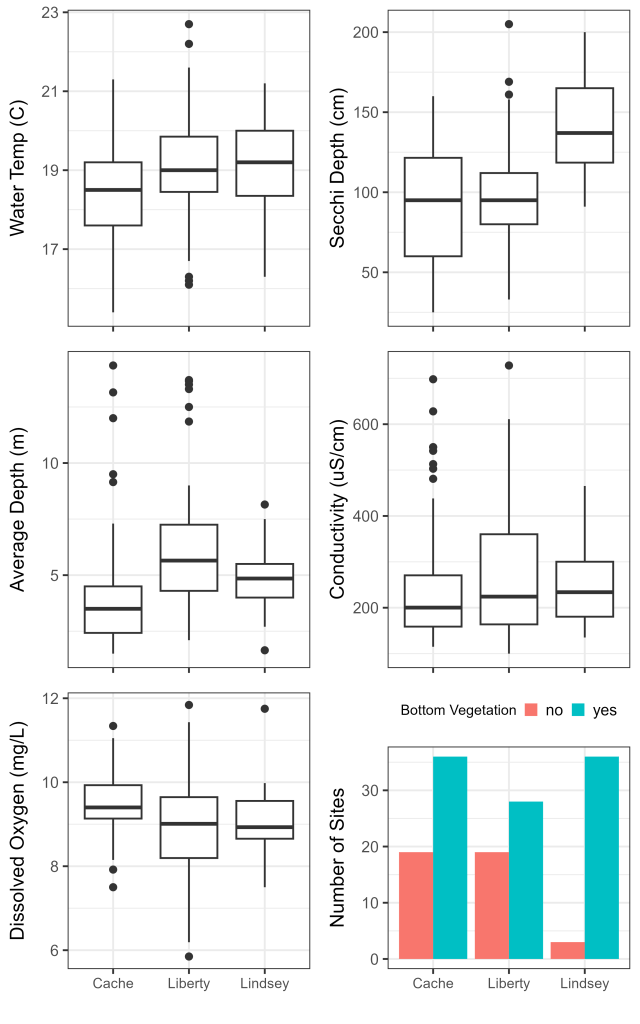
To investigate potential habitat differences between the subregions, we tested for associations between environmental variables and subregion using ANOVA, Kruskal-Wallis, Chi-Squared and pairwise post-hoc tests. We first used ANOVA to test for associations between subregion and the continuous environmental variables, including water temperature, Secchi depth, water depth, and dissolved oxygen. We inspected the residuals from the ANOVA models for normality using quantile-quantile plots and tested for normality using the Shapiro-Wilk test. We re-ran models that did not meet the assumption of normality using the non-parametric Kruskal-Wallis rank sum test. We then tested for an association between the single categorical predictor variable, presence of SAV, and subregion using a chi-squared test.

Once all subregional environmental models were completed, we ran post-hoc tests to examine the pairwise relationships amongst subregions. We used Tukey’s multiple comparison of means for ANOVA models, the Dunn Kruskal-Wallis multiple comparison method with Bonferroni correction for Kruskal-Wallis models, and multiple pairwise Chi-Squared tests for the chi-squared model. We plotted environmental variables as boxplots for continuous variables and as a bar chart for the presence of SAV, by subregion, to visualize differences in environmental conditions.

We then analyzed catch data to determine whether sampling intensity was sufficient to adequately represent the regional fish assemblage vulnerable to our gear. For this analysis we generated species accumulation curves for all North Delta samples as well as by strata (Lindsey complex, Cache complex, Liberty complex) and for paired day and night groupings using the community ecology package ‘vegan’ (vegan v.2.6-4, https://CRAN.R-project.org/package=vegan; accessed 13 Dec 2023) function ‘specaccum’ in the program R (R v.4.1.2, https://www.R-project.org/, accessed 13 Dec 2023). We generated species accumulation curves with the random accumulator method and ran the analysis for 100 permutations. We then estimated total species richness using the Chao (Chao 1987), Jacknife 1 and 2, and bootstrap methods (Walther and Morand 1998) using the ‘specpool’ function in the ‘vegan’ package. We report total species richness for all methods; however, the bootstrap method produced the most precise estimates based on standard errors and was primarily used to assess community representation. If measured species richness fell within a 95% confidence interval of the bootstrap estimate, we considered that grouping or stratum to be fully sampled.

The species richness estimation methods assume a closed species pool, which is a difficult assumption to meet in an open system such as the North Delta. We assume that the sampling timeframe allowed for potential contact with all species available, including both reproductive (migratory) and non-reproductive (non-migratory) individuals. We contacted all of those species most likely to migrate in and out of the North Delta, including Sacramento Splittail, Striped Bass, and American Shad (Alosa sapidissima). However, the possibility for rare and/or migratory individuals of other species to move in and out of our sampling area suggests that total species richness estimates are likely an underestimate of true species richness.

Once adequate sampling density had been determined, we tested the minimum sampling density required to represent different percentages of the total fish assemblage following the methods of Quist et al. (2007). We drew a total of 1,000 permutations of species richness without replacement for sampling densities from one netset up to the maximum number of netsets sampled for the North Delta and each of the individual subregions, using the ‘specaccum’ function in ‘vegan’. We then extracted the individual permutations from the species accumulation output and summed the number of occurrences where 100%, 90%, 80%, 70%, 60%, and 50% of the total sampled species richness was sampled for each sample size. We then divided these occurrences by 1000 to generate a probability of capturing 50–100% of the available fish assemblage for each sample size.

We standardized raw catch data as catch-per-unit-effort (CPUE), calculated as the number of fish caught per hour fishing using one complete gillnet (AFS experimental gillnet plus large fish gillnet). We calculated CPUE for all fish captured, by individual species, by subregion, by time of day (sampling period), and for native and introduced species. We then organized individual species CPUEs as a matrix, with species as columns and individual gillnet sets as rows, for use in ordination-based visualization and modeling.

We summarized length frequency data for all species captured during sampling by calculating the median, standard deviation, max, and minimum fork length. In addition, we visualized length frequencies for the two most frequently captured species, comparing their length frequency distributions to those observed in IEP trawl and seine surveys. We plotted length frequency as histograms of catch, using 10 mm bin widths. We sourced IEP trawl and seine data from the San Francisco Bay Study, Suisun Marsh Fish Study, Fall Midwater Trawl, Spring Kodiak Trawl, Delta Juvenile Fish Monitoring Study, Enhanced Delta Smelt Monitoring, 20 mm Survey, Smelt Larval Survey, and Summer Townet Survey using the aggregated “deltafish” dataset (deltafish v.0.1.0, https://delta-stewardship-council.github.io/deltafish/, accessed 13 Dec 2023; Bashevkin et al. 2022). Complete IEP data were not available for 2023, so we used 2019 data as a comparative year instead. Both 2019 and 2023 were classified as “wet” years by the CDWR with Sacramento Valley runoff of 24.77 million acre-feet (maf) and 24.11 maf, respectively (CDWR 2023), resulting in comparable hydrologic conditions.

We explored community assemblage data using non-metric multidimensional scaling (NMDS). NMDS is an ordination method that reduces multi-dimensional data into two or more orthogonal axes for plotting in two dimensions, allowing for comparison and assessment of communities in a spatial context. We square root transformed species CPUE to reduce the influence of common species and increase the relative influence of moderately abundant species (Brown and Michniuk 2007). We chose to use the Bray-Curtis dissimilarity metric (Bray and Curtis 1957) due to its ability to account for both species composition and abundance when comparing samples (Ricotta and Podani 2017) and omitted samples with zero catch for NMDS analyses. Additionally, we removed one “doubleton” record (catch occurrence with a species that was only captured twice) from the catch matrix for paired day/night samples due to its behavior as an outlier in the ordination. We then generated ordinations comparing North Delta subregions, vegetation state, and paired day and night samples using the function ‘metaMDS’ in ‘vegan’ (Oksanen et al. 2022), with 100 random starts. We calculated 95% confidence ellipsoids and applied them to NMDS plots to show the spatial clustering of points in relation to environmental metrics. We generated all figures using ggplot2 (ggplot2 v.3.4.1, https://ggplot2.tidyverse.org/, accessed 13 Dec 2023).

We tested the homogeneity of group dispersions for categorical predictor variables using the function ‘betadisper’ in ‘vegan’ to ensure proper inputs for permutational analysis of variance (PERMANOVA) modeling. Although PERMANOVA is generally insensitive to heterogeneous dispersions for balanced samples, bias may be introduced if unbalanced samples with heterogeneous dispersions are included in models (Anderson and Walsh 2013). We tested the predictor variables subregion, submersed aquatic vegetation, and tidal state. While the sampling design ensured balanced samples between day and night netsets within the paired samples, minimizing the risk of bias regardless of dispersion, we also tested the variable time of day for paired samples.

We then used PERMANOVA modeling to test for associations between community composition, time of day, subregion, and various environmental variables. We again omitted samples with zero catch. We chose to use PERMANOVA modeling due to its ability to handle and describe differences in abnormally distributed community data, which is often heavily zero-weighted (Lek et al. 2011; Anderson and Walsh 2013). We constructed models using the ‘adonis2’ function in the package ‘vegan’ (vegan v.2.6.4, https://rdrr.io/cran/vegan/, accessed 13 Dec 2023) using the square root of CPUE as the input matrix, the Bray-Curtis dissimilarity metric, and 999 random permutations. We ran two models – one to determine the association between community assemblage and subregion, presence of SAV, water temperature (C), Secchi depth (cm), water depth (m), and dissolved oxygen (mg/L) for all samples, and another to examine the association between community assemblage and time of day and Secchi depth (cm) for only those paired day and night samples. We selected environmental predictor variables based on ecological relevance to fish species abundance and distribution. To identify drivers of significant relationships for categorical predictors with more than two categories we used pairwise PERMANOVA testing using ‘pairwise.adonis2’ in the ‘pairwiseAdonis’ package (pairwiseAdonis v.0.4.1, https://github.com/pmartinezarbizu/pairwiseAdonis, accessed 12 Dec 2023). We applied a Bonferroni correction to pairwise PERMANOVA results to reduce Type 1 error.

Data from this study are available from: https://doi.org/10.6073/pasta/befa271d32e9ab2ae7919930f937d8fb

Results

Environmental models indicated differences in water temperature (ANOVA: F₂ = 4.45, P = 0.013), Secchi depth (ANOVA: F₂ = 26.28, P < 0.001), water depth (Kruskal-Wallis: χ²₂ = 24.26, P < 0.001), dissolved oxygen (Kruskal-Wallis: χ²₂ = 12.22, P = 0.002), and the presence of SAV (Chi-Squared: χ²₂ = 136.19, P < 0.001) between the subregions (Fig. 3). From the pairwise comparisons, water temperature was cooler in the Cache Complex than either the Liberty (diff = 0.72 ± 0.65°C, P = 0.027) or Lindsey (diff = 0.71 ± 0.69°C, P = 0.042) Complexes, Secchi depth was higher in the Lindsey Complex than in either the Cache (diff = 48.39 ± 16.81 cm, P < 0.001) or Liberty (diff = 43.18 ± 17.39cm, P < 0.001) Complexes, water depth was shallower in the Cache Complex than in Lindsey (Z = -2.97, P = 0.008) or Liberty (Z = -4.83, P < 0.001) Complexes, and the Cache Complex had higher dissolved oxygen than either the Lindsey (Z = 2.87, P = 0.012) or Liberty (Z = 3.05, P = 0.007) Complexes. Differences in presence of SAV existed for all pairwise comparisons (χ²₁ = 88.50, P < 0.001).

A total of 572 fish were captured in 141 netsets. We captured 16 species, including 191 Striped Bass (14.5 – 67.7 cm FL, median = 33.3 cm FL; Table 1), 152 Sacramento Hitch (13–38.7 cm FL, median = 24.5 cm FL; Table 1), and 62 White Catfish (Ameiurus catus; 16.0–46.4 cm FL, median = 23.1 cm FL; Table 1), amongst others (Table 2). Sampling occurred between 2 May and 21 June 2023. Of the 572 fish captured, we released 416 with PIT tags, including 118 Sacramento Hitch, 113 Striped Bass, and 59 White Catfish (Table 2). Approximately 70% of captured fish were released in good condition, 18% in fair condition, 7% in poor condition, and 5% were dead when released. Through collaboration with the CVSMP, an additional 2,810 Striped Bass (26.0–119.0 cm FL, median = 42.0 cm FL) were tagged with PIT tags between 16 March and 18 April 2023, from fyke traps deployed in the Lower Sacramento River. The YBFMP did not catch any target species and the SMFS scanned a portion of captured adult Sacramento Splittail but was unable to deploy any tags due to time constraints. Six PIT tags deployed by the CVSMP were recaptured from CVSMP fyke traps, most within one month of release. No PIT tags were recaptured during gillnet or SMFS sampling.

Table 1. Median, standard deviation, minimum, and maximum fork length for each species captured in this study, measured in millimeters. Species ordered by frequency of catch.

Common Name	Median FL	Standard Deviation	Min	Max
Striped Bass	333	110.3	145	677
Sacramento Hitch	245	52.9	130	387
White Catfish	231	52.1	160	464
Sacramento Splittail	326	39.5	161	379
Largemouth Bass	248	77.6	130	417
Sacramento Pikeminnow	261	131.0	182	518
Tule Perch	148	26.5	135	251
Redear Sunfish	165	39.4	125	279
Golden Shiner	146	21.3	124	178
Sacramento Sucker	431	118.8	233	565
Threadfin Shad	118	17.2	113	166
Common Carp	264	52.2	192	347
Black Crappie	218	67.8	103	311
Bluegill Sunfish	146	32.9	101	165
American Shad	152	N/A	152	152
Channel Catfish	528	N/A	528	528

Table 2. Species names, species codes, status (native vs. introduced), total catch, catch by subregion, and number of PIT tags deployed for each fish species encountered in North Delta gillnet sampling. 141 netsets were conducted in total, 55 netsets were conducted in the Cache Complex, 47 in the Liberty Complex, and 39 in the Lindsey Complex.

Common Name	Species Code	Status	Total Catch	Cache Complex Catch	Liberty Complex Catch	Lindsey Complex Catch	Number PIT Tagged
Striped Bass	STRBAS	non-native	191	99	58	34	110
Sacramento Hitch	HITCH	native	152	112	29	11	118
White Catfish	WHICAT	non-native	62	23	33	6	59
Sacramento Splittail	SPLITT	native	47	26	20	1	41
Largemouth Bass	LARBAS	non-native	24	8	5	11	15
Sacramento Pikeminnow	SACPIK	native	21	7	10	4	17
Tule Perch	TULPER	native	18	3	8	7	16
Redear Sunfish	REDEAR	non-native	12	4	2	6	10
Golden Shiner	GOLSHI	non-native	9	7	0	2	3
Sacramento Sucker	SACSUC	native	9	8	1	0	9
Threadfin Shad	THRSHA	non-native	9	8	0	1	0
Common Carp	COMCAR	non-native	7	3	4	0	7
Black Crappie	BLACRA	non-native	6	4	2	0	4
Bluegill Sunfish	BLUGIL	non-native	3	1	1	1	2
American Shad	AMESHA	non-native	1	0	1	0	0
Channel Catfish	CHACAT	non-native	1	1	0	0	1

Species accumulation curves for all samples from the North Delta (n = 141), Cache Slough Complex (n = 55), Lindsey Slough Complex (n = 39), Liberty Complex (n = 47), and for paired day (n = 33) and night (n = 33) samples all appeared to reach or nearly reach an asymptote, indicating adequate representation of the available fish community (Fig. 4). Likewise, species richness from all sampled strata fell within a 95% confidence interval of the bootstrap estimate of total species richness (Table 3). As such, each stratum was considered adequately sampled and included in PERMANOVA models as predictor variables.

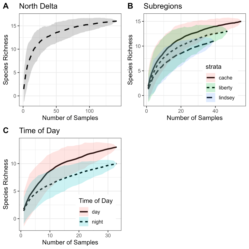
Table 3. Estimated total species richness for each survey substrata. Strata were considered fully sampled if the number of species captured (Species) was within 1.96*boot.se of the bootstrapped (boot) species richness estimate. Species is the total number of species detected, “Chao” is the Chao estimate of total species richness, “jack1” is the jackknife1 estimate of total species richness, “jack2” is the jackknife2 estimate of total species richness, “boot” is the bootstrap estimate of total species richness, and “n” is the total number of samples included. Columns ending with “.se” are the standard error of the associated estimate.

Region	Species	Chao	Chao.se	jack1	jack1.se	jack2	boot	boot.se	n
North Delta	16	18.0	3.7	18.0	1.4	19.0	16.9	0.8	141
Cache Complex	15	19.4	7.1	17.9	1.7	19.9	16.3	1.0	55
Lindsey Complex	11	16.8	7.0	14.9	1.9	18.7	12.6	1.1	39
Liberty Complex	13	15.2	3.3	15.9	2.2	16.9	14.5	1.3	47
Day	13	16.9	5.1	16.9	1.9	18.8	14.7	1.2	33
Night	10	17.8	11.3	13.9	1.9	16.7	11.6	1.0	33

The minimum required sampling as determined through permutational probabilities showed similar probability curves for detecting 50–100% of species for the three sub-regions, with higher sampling intensities required for the entire North Delta (Fig. 5). To achieve a 95% probability of detecting 50–100% of available species, the North Delta required 18 to 138 samples, the Cache Complex required 15 to 55 samples, the Liberty Complex required 18 to 46 samples, and the Lindsey Complex required 17 to 39 samples to capture 50 to 100% of available species, respectively (Table 4).

Table 4. Total sample size (n) and number of samples required to capture 50–100% of the available species assemblage, with 95% probability.

Subregion	n	100%	90%	80%	70%	60%	50%
North Delta	141	138	114	62	48	30	18
Cache Complex	55	55	48	31	25	18	15
Liberty Complex	47	46	45	38	32	23	18
Lindsey Complex	39	39	35	30	24	20	17

The Cache Slough Complex had the highest median CPUE for all species (3.1 fish/hr), followed by the Liberty Island Complex (1.8 fish/hr) and the Lindsey Slough Complex (1.0 fish/hr; Fig. 6). Likewise, maximum overall CPUE was highest in the Cache Slough Complex (40.0 fish/hr), followed by the Liberty Island Complex (14.5 fish/hr) and Lindsey Slough Complex (9.8 fish/hr; Fig. 6). Median native fish CPUE was considerably greater in the Cache Slough Complex (1.0 fish/hr) than in either the Liberty Island Complex (0 fish/hr) or the Lindsey Slough Complex (0 fish/hr; Fig. 6). The disparity in native fish catch was driven by the exceptionally high catch of Sacramento Hitch in the Cache Slough Complex, which was the most frequently encountered and highest CPUE species in the subregion (Table 2; Fig. 7). Median CPUE of non-native fishes was also greatest in the Cache Slough Complex (2.0 fish/hr), followed by the Lindsey Slough Complex (1.0 fish/hr) and the Liberty Island Complex (0.97 fish/hr; Fig. 6). All subregions had higher median CPUEs for non-native species than for native species (Fig. 6), driven in part by the high catch of Striped Bass, which were the most common species contacted over the survey (Table 2; Fig. 7).

Fish captured in our study were substantially larger than those captured in the trawl- and seine-based surveys of the IEP, as shown through length frequency histograms (Fig. 8). While the overall catch of Striped Bass was an order of magnitude larger amongst the IEP trawl/seine surveys, the sizes of Striped Bass captured were primarily less than 150mm FL. In contrast, our samples were primarily of Striped Bass larger than 150mm, with lengths extending up to 677mm FL (Table 1; Fig. 8). Two clear age classes are visible in the IEP Striped Bass length frequency, likely representing age 0 and age 1 individuals, while 4–5 age classes from age 2 to age 5 or 6 exist within our samples (Fig. 8). For Sacramento Hitch, IEP trawl/seine catch consisted mostly of fish smaller than 100 mm FL, whereas our study sampled Sacramento Hitch between 130 and 387 mm FL (Table 1; Fig. 8). Despite the difference in overall sampling effort between our study (141 samples) and the IEP trawl/seine surveys (17,093 samples), more Sacramento Hitch were caught in our samples.

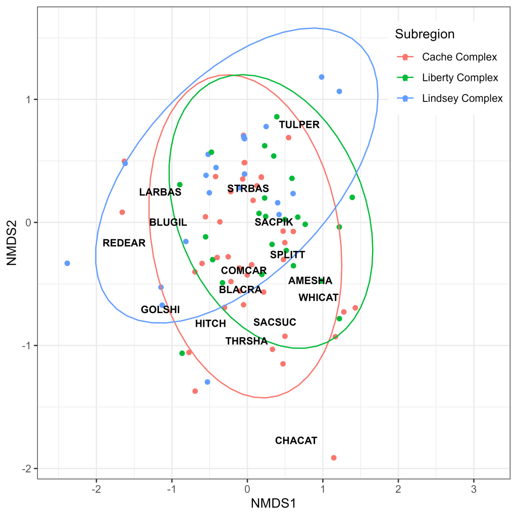
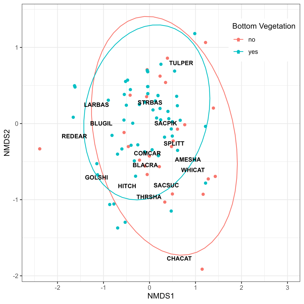
Ordination analysis revealed considerable overlap in assemblage composition between subregions, with highly similar 95% confidence ellipsoids in the Cache Slough and Liberty Island Complexes (Fig. 9). The Lindsey Slough Complex displayed the most distinct clustering but still exhibited considerable overlap (Fig. 9). Generally, species clustered according to their phylogenies, with the centroids of distribution for most centrarchids (Largemouth Bass, Redear Sunfish [Lepomis microlophus], Bluegill Sunfish [Lepomis macrochirus]) and cyprinids (Golden Shiner [Notemigonus crysoleucas], Sacramento Hitch, Common Carp [Cyprinus carpio], Sacramento Splittail, Sacramento Pikeminnow) clustering in relatively close proximity to one another (Fig. 9). While the centroids of species typically associated with SAV (Largemouth Bass, Redear Sunfish, Bluegill Sunfish, Golden Shiner) appeared to cluster together, there was a high degree of overlap between the 95% confidence ellipsoids for sites with and without SAV present in the net path (Fig. 10). The ellipsoid for sites without SAV was larger than that for sites with SAV; however, this may have been driven by a single outlier catch of Channel Catfish (Ictalurus punctatus; Fig. 10), a species only encountered on a single occasion (Table 2).

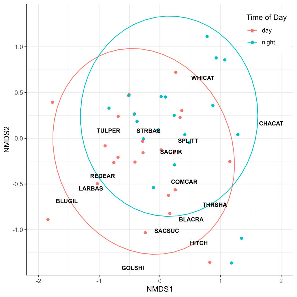
Species composition was similar between day and night paired samples, with slight deviations in 95% confidence ellipsoids apparently driven in part by increased catch of catfish species during night sets and SAV associated species (Bluegill Sunfish, Largemouth Bass, Golden Shiner) during day sets (Fig. 11). The centroid of Striped Bass, the most captured species (Table 2), was located near the center of both ellipses (Fig. 11), indicating good representation in both day and night sets. In contrast, the centroid of Sacramento Hitch, the second most captured species (Table 2), was outside the night set ellipse (Fig. 11), indicating poor representation of this species from night sets.

Betadispersion tests showed homogeneous spread for the categorical variables Subregion and Presence of SAV for the full model and time of day for the paired model. Conversely, Tidal State displayed heterogeneous spread amongst the ebb, flood, and slack groups. While PERMANOVA is typically insensitive to heterogeneous spread given balanced samples, there were considerably more samples collected during “flood” conditions (n = 55) than in “ebb” (n = 41) or “slack” conditions (n = 8), so this variable was omitted from the full PERMANOVA model.

PERMANOVA results indicated effects of subregion (F₂ = 2.26, P = 0.010), Secchi depth (F₁ = 2.47, P = 0.030), and average depth (F₁ = 4.19, P = 0.003) from samples collected in the North Delta (Table 5). There may have also been an effect of submersed aquatic vegetation (F₁ = 1.97, P = 0.079), although, it did not meet the commonly used arbitrary significance cutoff of α = 0.05. There was no effect of water temperature (F₁ = 0.87, P = 0.495) or dissolved oxygen (F₁ = 0.95, P = 0.447). From the day/night paired model, effects were indicated for both time of day (F₁ = 3.09, P = 0.014) and Secchi depth (F₁ = 2.60, P = 0.035; Table 6). Pairwise comparisons from the full model did not reveal any differences in assemblage between the Cache Slough Complex and Lindsey Slough Complex (F₁ = 2.30, adjusted-P = 0.123), the Liberty Island Complex and Lindsey Slough Complex (F₁ = 2.14, adjusted-P = 0.192), or the Cache Slough Complex and Liberty Island Complex (F₁ = 1.97, adjusted-P = 0.270).

Table 5. PERMANOVA model results on the effects of subregion, submersed aquatic vegetation (bottom vegetation), water temperature, Secchi depth, average depth, and dissolved oxygen for samples collected in the North Delta gillnet sampling.

Variable	df	Sum of Squares	R2	F	P-value
Subregion	2	1.20	0.04	2.26	0.010
Bottom Vegetation	1	0.52	0.02	1.97	0.079
Water Temperature	1	0.23	0.01	0.87	0.495
Secchi Depth	1	0.66	0.02	2.47	0.030
Average Depth	1	1.12	0.04	4.19	0.003
Dissolved Oxygen	1	0.25	0.01	0.95	0.447
Residual	96	25.57	0.87	N/A	N/A
Total	103	29.56	1.00	N/A	N/A

Table 6. PERMANOVA model results on the effects of time of day (day/night) and Secchi depth on fish composition for paired samples collected in the North Delta gillnet sampling.

Variable	df	Sum of Squares	R2	F	P-value
Time of Day	1	0.76	0.06	3.09	0.014
Secchi Depth	1	0.64	0.05	2.60	0.035
Residual	45	11.02	0.89	N/A	N/A
Total	47	12.41	1.00	N/A	N/A

Discussion

The results from this study demonstrate the utility and feasibility of this sampling methodology for describing large fish assemblages as well as its ability to integrate with existing IEP and CDFW surveys. We met our objectives by determining the sampling intensity required to fully represent the fish assemblages of the North Delta and its three subregions, quantifying diel effects on species representation, and assessing the feasibility of using PIT tagging from an assemblage-focused gillnet study to estimate species abundance. Additionally, we effectively catalogued the springtime large fish assemblage of the North Delta under wet conditions and demonstrated the differences in length frequency between fishes captured in experimental gillnets and those from IEP trawl- and seine-based surveys. These findings support the continued use of gillnet sampling to more comprehensively represent the fish assemblage of the SFE.

The number of samples required to capture 50% of the available species ranged from 15–18, while capturing 100% of the available species required 39-138, depending on the region/subregion (Table 4; Fig. 5). While full species representation is ideal, it may not be necessary depending on management goals, especially if impacts to sensitive species are a concern. Gillnets result in relatively high levels of damage to captured fishes compared to less invasive capture techniques, as shown by the 30% of fish that were in fair, poor, or dead condition upon release. Mortality rates (immediate or delayed) from gillnets vary by species (Broadhurst et al. 2008), with species such as salmonids being sensitive to capture and others such as sturgeon being largely insensitive (Stompe et al. 2022). When sensitive species are present, as is the case during the fall and spring when Chinook Salmon return to Central Valley rivers to spawn, lower levels of assemblage representation may be targeted to limit incidental mortality. Reducing the species coverage to 80% lowered the required number of samples to 30-38 for the subregions and 62 for the entire North Delta. Reducing effort to this level (eight sampling days assuming eight netsets per day) would likely miss infrequently captured species such as Channel Catfish (n = 1), American Shad (n = 1), and Bluegill Sunfish (n = 3), but would increase survey efficiency in detecting the species that are most abundant and/or most available to gillnet gear. A reduction in sampling intensity would also make available more resources to sample other regions, increasing the overall spatial coverage of the survey.

Perhaps the most encouraging result from this study was the exceptional catch of Sacramento Hitch. Sacramento Hitch is a native cyprinid species that is not frequently encountered in most trawl- or seine-based IEP surveys (Fig. 8), potentially due to poor gear efficiency or a lack of spatial overlap, as relatively little sampling by trawl- and seine-based IEP surveys occurs in the areas sampled in this study. Additionally, this species has been identified by CDFW as a species of moderate concern, with data limitations but probable declines throughout their range (CDFW 2015). The high catch of Sacramento Hitch in this study indicates either extremely high gear efficiency, or more likely, a relatively large population of Sacramento Hitch in the North Delta which is supported by recent electrofishing studies (MacFarland et al. 2022; Williamshen et al. 2023). Furthermore, the wide range of sizes contacted (Fig. 8) indicates that the population is not supported by a single strong year class, but rather there are several year classes present, and that successful spawning is happening annually across a range of precipitation and outflow conditions. This somewhat contradicts findings from recent electrofishing studies in the North Delta, which found primarily juvenile Sacramento Hitch in this region and low densities of adults in other parts of the Delta (MacFarland et al. 2022). This suggests that gillnets may be more efficient at catching larger individuals or that the age composition of Sacramento Hitch in the North Delta has changed between the time when the data from MacFarland (2022) were collected (2018–2021) and this study (2023). Additionally, Sacramento Hitch were not a dominant species in recent (2017–2018) gillnetting efforts in nearby North Delta habitats (Clause et al. 2024), indicating that the observed high abundance of adults in this study may be a relatively recent phenomenon.

Conversely, a discouraging result of this study was the lack of White Sturgeon (Acipenser transmontanus) catch. White Sturgeon is a benthically associated, long-lived, and late maturing fish species, a California species of special concern, and at the time of this writing, is the subject of both the federal Endangered Species Act and California Endangered Species Act listing petitions. While adult White Sturgeon are likely strong enough to break free from the relatively light monofilament that makes up AFS experimental gillnets, juvenile and subadult individuals should be easily retained if they were to be entangled in this gear. It is possible that our gillnets have a low capture efficiency for White Sturgeon due to the anchored (fixed) set methodology which relies on fish to actively swim into the net. However, given the demonstrated catch of subadult White and the closely related Green Sturgeon (Acipenser medirostris) in nearby downstream habitats (M. Beccio, personal communication) by anchored gillnets, this explanation seems unlikely. The lack of White Sturgeon catch in our study is consistent with previous gillnetting efforts using experimental gillnets in the North Delta, which captured only two White Sturgeon from 670 netsets in 2017 and 2018 (Steinke et al. 2019). These findings suggest that White Sturgeon do not frequent the habitats of the North Delta and instead spend their time in other parts of the estuary.

Despite not catching sturgeon, we were able to effectively extend the size range of fishes sampled beyond what is captured in IEP trawl- and seine-based surveys (Fig. 8). The implications of this are evident for species such as Striped Bass, which are predominately represented by two age classes (age-0, age-1) in the IEP trawl/seine data. While metrics of age-0 and age-1 abundance are important for determining juvenile recruitment, they cannot fully explain trends in overall species abundance (Kimmerer et al 2000). In addition, these data alone cannot quantify the number of adults available to function as predators or to contribute to the recreational fishery. While not as long lived as Striped Bass, this concept also applies to other species such as Sacramento Hitch and Sacramento Splittail that reach relatively large sizes but are not well represented as adults by IEP trawl/seine surveys.

While we successfully deployed over 3,000 PIT tags between our study and the CVSMP, the within-season recapture rates were insufficient to calculate abundance or describe the movement dynamics of any given species. This outcome can be partly explained by the directionality of the Striped Bass spawning migration and the use of fyke traps in the Sacramento River, which accounts for the fish tagged by the CVSMP. Striped Bass are only vulnerable to fyke traps when moving upriver to spawn, after which they will not become available to the gear until the next spawning migration approximately one year later. Likewise, individuals tagged in the Sacramento River are unlikely to redistribute to the North Delta until the spawning period had commenced—typically in May or June (Goertler et al. 2021). The efficacy of mark-recapture for estimating abundance would become clearer after two or more years of sampling have elapsed and tagged fish have sufficiently mixed within their greater populations. However, the sampling intensity required to deploy and recover enough tags is likely not practical for an assemblage-type study like this one. Additionally, the open and dynamic nature of the Delta is generally not compatible with the assumptions of most mark-recapture models, further complicating the implementation of this methodology in any future large-fish assemblage monitoring.

There was a high degree of assemblage overlap between the three subregions, with the Lindsey Slough Complex standing out as the most distinct (Fig. 9). The Lindsey Slough Complex was also relatively depauperate, both in terms of total catch (Fig. 6) and species diversity (Fig. 7). These subtle differences are likely driven by the increased catch of some SAV-associated fishes such as Golden Shiner and Redear Sunfish in the Lindsey Slough Complex along with the absence of Sacramento Sucker, Common Carp, Black Crappie (Pomoxis nigromaculatus), American Shad, and Channel Catfish (Fig. 7). These observations are supported by model results, which indicate potential effects of SAV on species assemblage (Table 5), as well as significantly more sites with SAV and clearer water (increased Secchi depth) in the Lindsey Slough Complex (Fig. 3). Given this, the somewhat different assemblage composition (Fig. 9) and reduced catch in the Lindsey Slough Complex (Figs. 6, 7) may be driven by preferences of some species for turbid and less highly vegetated habitats, increased net avoidance behavior in areas with higher Secchi depth, or a combination of both factors.

On the opposite end of the spectrum, the Cache Slough Complex had the highest diversity, and the highest overall, native, and introduced species catches amongst the three subregions (Figs. 6, 7), highlighting the importance of this region in supporting North Delta fish biomass. High catches in the Cache Slough Complex may be linked to the fact that this subregion was significantly shallower, more turbid, and less vegetated than either Liberty Island or Lindsey Slough Complexes (Fig. 3). These differences in overall catch and diversity should be considered when evaluating regions for modification, as actions in the Cache Slough Complex may have outsized effects on the native species that occur there. Likewise, conditions in the Lindsey Slough Complex could potentially be improved to better support native fish and fishes in general, potentially by emulating the environmental conditions found in the Cache Slough Complex.

When considering day and night paired samples, PERMANOVA modeling indicated that the assemblages caught during each time period are not duplicative of one another. The significant result for both time of day and turbidity (measured as Secchi depth) suggests that both fish activity and net avoidance behavior or turbidity preference may play a role. Because samples were paired and collected within approximately five hours of one another, there should be minimal interaction between turbidity and time of day. While we cannot definitively determine from these data whether fish activity or net avoidance is responsible for the significant result of Secchi depth in both this and the full model, we can use the effect of time of day to elucidate that fish activity does change and influences gillnet catch.

When using these results to inform future study designs, we may examine the ordination plot for day versus night samples to guide our approach. The ordination plot indicates that the only two species with centroids more closely aligned with night sampling are White Catfish and Channel Catfish. In contrast, Bluegill Sunfish, Largemouth Bass, Sacramento Hitch, Sacramento Sucker, and Black Crappie were all outside of the 95% confidence ellipsoid for night sets but within the day ellipsoid. If the goal is to target catfish species, say, to examine the distribution of benthic predators, night sampling has clear advantages. However, if management questions are focused on species such as Bluegill Sunfish, Largemouth Bass, Sacramento Hitch, Sacramento Sucker, and Black Crappie, then day samples are the superior choice. A hybrid approach incorporating both day and night sets would result in the best overall assemblage representation. Regardless of which species are best represented between the two sampling periods, it is important to note that night sampling is logistically much more challenging, introducing higher levels of risk to crews and requiring specialized equipment such as radar and high-powered flood lights.

It should also be noted that the results of this study were limited to the relatively cool and high turbidity months of April through June, during a year classified as “wet” in the Sacramento River basin (CDWR 2023). Given this, the association between species assemblages and environmental variables including temperature, turbidity, dissolved oxygen, and presence of SAV may change under drier conditions or during the summer and fall months when water conditions are warmer and clearer, and when SAV densities are highest. These seasonal differences in environmental conditions may also result in changes in distribution of large and mobile species (e.g., Striped Bass) as well as changes in diel activity levels. Any future IEP monitoring studies (utilizing gillnets or otherwise) that aim to describe species assemblages should consider the seasonal effects of environmental variables and should iteratively analyze assemblage representation to maximize survey efficiency.

Overall, we demonstrated the number of samples required to represent different percentages of the total available large fish assemblage, the benefits and disadvantages of sampling with gillnets during night hours, and the limitations of mark recapture in surveys not specifically targeting single species (at least on the scale of several months). We also expanded SFE fish sampling to include the large fish assemblages in many habitats not accessible to electrofishing gear, establishing another year of assemblage information in the North Delta for comparison with past and future gillnet efforts. Based on our findings, future sampling that is limited to day sampling with at least 62 and up to 138 samples per region could describe 80–100% of the available fish assemblage which could be useful in answering key management questions.

Acknowledgements

Thank you to the dedicated field staff, including Analicia Ortega, Joshua Canepa-Gallo, Zachary Liddle, and Taryn Mitoma, who made the field data collection possible. We would also like to thank Brian Schreier and Daphne Gill, who provided valuable input in the conception and design of this study. Brian Schreier, Rosemary Hartman, and Alicia Seesholtz provided useful edits of this manuscript as did two anonymous reviewers. This study was funded by the Department of Water Resources as part of the Interagency Ecological Program.

Literature Cited

• Aasen, G., and J. Morinaka. 2018. Fish salvage at the State Water Project’s and Central Valley Project’s fish facilities during the 2017 water year. IEP Newsletter 31(1):3–9. Available from: https://filelib.wildlife.ca.gov/Public/salvage/Annual%20Salvage%20Reports/2017%20IEP%20Water%20Year%20Salvage%20report.pdf
• Aasen, G., and W. Griffiths. 2022. Fish salvage at the Tracy fish collection facility during the 2021 water year. California Department of Fish and Wildlife, Stockton, CA, USA. Available from: https://filelib.wildlife.ca.gov/Public/salvage/Annual%20Salvage%20Reports/2021%20TFCF%20Salvage%20Annual%20Report%20Final.pdf
• Anderson, M. J., and D. C. Walsh. 2013. PERMANOVA, ANOSIM, and the Mantel test in the face of heterogeneous dispersions: what null hypothesis are you testing? Ecological Monographs 83(4):557–574. https://doi.org/10.1890/12-2010.1
• Bashevkin, S. M, J. W. Gaeta, T. X. Nguyen, L. Mitchell, and S. Khanna. 2022. Fish abundance in the San Francisco Estuary (1959–2021), an integration of 9 monitoring surveys. ver 1. Environmental Data Initiative. https://doi.org/10.6073/pasta/0cdf7e5e954be1798ab9bf4f23816e83
• Brandl, S., B. Schreier, J. L. Conrad, B. May, and M. Baerwald. 2021. Enumerating predation on Chinook Salmon, Delta Smelt, and other San Francisco Estuary ffishes using genetics. North American Journal of Fisheries Management 41(4):1053–1065. https://doi.org/10.1002/nafm.10582
• Bonar, S. A., W. A. Hubert, and D. W. Willis. 2009. Standard Methods for Sampling North American Freshwater Fishes. American Fisheries Society, Bethesda, MD, USA.
• Bray, J. R., and J. T. Curtis. 1957. An ordination of the upland forest communities of southern Wisconsin. Ecological Monographs 27(4):326–349. https://doi.org/10.2307/1942268
• Broadhurst, M. K., R. B. Millar, C. P. Brand, and S. S. Uhlmann. 2008. Mortality of discards from southeastern Australian beach seines and gillnets. Diseases of Aquatic Organisms 80(1):51–61.
• Brown, L. R., and D. Michniuk. 2007. Littoral fish assemblages of the alien-dominated Sacramento-San Joaquin Delta, California, 1980–1983 and 2001–2003. Estuaries and Coasts 30:186–200. https://doi.org/10.1007/BF02782979
• Calhoun, A. J. 1952. Annual migrations of California striped bass. California Fish and Game 38:391–404.
• California Department of Fish and Wildlife (CDFW). 2015. Sacramento Hitch Lavinia exilicauda exilicauda (Baird and Girard). California Department of Fish and Wildlife. Sacramento, CA, USA. Available from: https://nrm.dfg.ca.gov/FileHandler.ashx?DocumentID=104368&inline
• California Department of Fish and Wildlife (CDFW). 2020. Long-term operation of the state water project in the Sacramento San Joaquin Delta. Incidental Take Permit No. 2081-2019-066-00. California Department of Fish and Wildlife. Sacramento, CA, USA.
• California Department of Water Resources (CDWR). 2023. Chronological reconstructed Sacramento and San Joaquin Valley water year hydrologic classification indices. California Department of Water Resources, Sacramento, CA, USA. Available from: https://cdec.water.ca.gov/reportapp/javareports?name=WSIHIST
• Chao, A. 1987. Estimating the population size for capture-recapture data with unequal catchability. Biometrics 43(4):783–791. https://doi.org/10.2307/2531532
• Clause, J. K, M. J. Farruggia, F. Feyrer, and M. J. Young. 2024. Wetland geomorphology and tidal hydrodynamics drive fine-scale fish community composition and abundance. Environmental Biology of Fishes 107:33–46. https://doi.org/10.1007/s10641-023-01507-w
• Cohen, A. N. and J. T. Carlton. 1998. Accelerating invasion rate in a highly invaded estuary.Science 279:555–558. https://doi.org/10.1126/science.279.5350.555
• Conomos, T. J., R. E. Smith, and J. W. Gartner. 1985. Environmental setting of San Francisco Bay. Pages 1–12 in J. E. Cloern and F. H. Nichols, editors. Temporal Dynamics of an Estuary: San Francisco Bay. Kluwer Boston Inc., Hingham, MA, USA.
• Crain, P. K. and P. B. Moyle. 2011. Biology, history, status and conservation of Sacramento perch, Archoplites interruptus. San Francisco Estuary and Watershed Science 9(1). https://doi.org/10.15447/sfews.2011v9iss1art5
• Feyrer, F., J. Hobbs, S. Acuna, B. Mahardja, L. Grimaldo, M. Baerwald, R. C. Johnson, and S. Teh. 2015. Metapopulation structure of a semi-anadromous fish in a dynamic environment. Canadian Journal of Fisheries and Aquatic Sciences 72(5):709–721. https://doi.org/10.1139/cjfas-2014-0433
• Goertler, P., B. Mahardja, and T. Sommer. 2021. Striped bass (Morone saxatilis) migration timing driven by estuary outflow and sea surface temperature in the San Francisco Bay-Delta, California. Scientific Reports 11(1):1–11. https://doi.org/10.1038/s41598-020-80517-5
• Honey, K., R. Baxter, Z. Hymanson, T. Sommer, M. Gingras, and P. Cadrett. 2004. IEP long-term fish monitoring program element review. Interagency Ecological Program, State of California, Sacramento, CA, USA. Available from: https://www.google.com/url?sa=t&rct=j&q=&esrc=s&source=web&cd=&ved=2ahUKEwjF7vq_oa-IAxVF0gIHHT4kEB8QFnoECBYQAQ&url=https%3A%2F%2Fnrm.dfg.ca.gov%2FFileHandler.ashx%3FDocumentID%3D32965&usg=AOvVaw029qw2-dTaPB8051eChs-N&opi=89978449
• Huntsman, B. M., M. J. Young, F. V. Feyrer, P. R. Stumpner, L. R. Brown, and J. R. Burau. 2023. Hydrodynamics and habitat interact to structure fish communities within terminal channels of a tidal freshwater delta. Ecosphere 14(1). https://doi.org/10.1002/ecs2.4339
• Interagency Ecological Program (IEP) Drought Synthesis Team. 2023. Ecological Impacts of Drought on Suisun Bay and the Sacramento-San Joaquin Delta with special attention to the extreme drought of 2020-2022. IEP Technical Report #100. Interagency Ecological Program for the San Francisco Estuary, Sacramento, CA, USA.
• Kimmerer, W. J., J. H. Cowan, L. W. Miller, and K. A. Rose. 2000. Analysis of an estuarine striped bass (Morone saxatilis) population: influence of density-dependent mortality between metamorphosis and recruitment. Canadian Journal of Fisheries and Aquatic Sciences 57(2):478–486. https://doi.org/10.1139/f99-273
• Klein, Z. B., M.C. Quist, A. M. Dux, and M. P. Corsi. 2019. Size selectivity of sampling gears used to sample kokanee. North American Journal of Fisheries Management, 39(2):343–352. https://doi.org/10.1002/nafm.10272
• Kohlhorst, D. W. 1980. Recent trends in the white sturgeon population in California’s Sacramento-San Joaquin Estuary. California Fish and Game 66:210–219.
• Lek, E., D. V. Fairclough, M. E. Platell, K. R. Clarke, J. R. Tweedley, and I. C. Potter. 2011. To what extent are the dietary compositions of three abundant, co‐occurring labrid species different and related to latitude, habitat, body size and season? Journal of Fish Biology 78(7):1913–1943. https://doi.org/10.1111/j.1095-8649.2011.02961.x
• Lund, J., E. Hanak, and W. Fleenor. 2007. Envisioning futures for the Sacramento-San Joaquin Delta. Public Policy Institute of California, San Francisco, California. Available from: https://www.ppic.org/wp-content/uploads/content/pubs/report/R_207JLR.pdf
• Martinez-Andrade, F. 2018. Trends in relative abundance and size of selected finfishes and shellfishes along the Texas coast: November 1975–December 2016. Management Data Series No. 291. Texas Parks and Wildlife, Coastal Fisheries Division, Austin, TX, USA. Available from: https://texashistory.unt.edu/ark:/67531/metapth1203651/
• McKenzie, R., and B. Mahardja. 2021. Evaluating the role of boat electrofishing in fish monitoring of the Sacramento–San Joaquin Delta. San Francisco Estuary and Watershed Science 19(1). https://doi.org/10.15447/sfews.2021v19iss1art4
• McKenzie, R., J. Speegle, A. Nanninga, E. Holcombe, J. Stagg, J. Hagen, E. Huber, G. Steinhart, and A. Arrambide. 2022. Interagency Ecological Program: USFWS Delta Boat Electrofishing Survey, 2018-2022 ver 3. Environmental Data Initiative. https://doi.org/10.6073/pasta/4886dbb80cf709a4c6e5906ff94eacdc
• Maryland Department of Natural Resources (MDNR). 2021. Chesapeake Bay Finfish Investigations. Report Number F-61-R-16. Maryland Department of Natural Resources, Annapolis, MD, USA. Available from: https://dnr.maryland.gov/fisheries/Documents/Final%20Report%20F-61-R-16%202020-2021.pdf
• Moyle, P. B., 2002. Inland Fishes of California: Revised and Expanded. University of California Press, Berkeley, CA, USA.
• Nobriga, M. L., and W. E. Smith. 2020. Did a shifting ecological baseline mask the predatory effect of Striped Bass on Delta Smelt? San Francisco Estuary and Watershed Science 18(1). https://doi.org/10.15447/sfews.2020v18iss1art1
• O’Connell, M. T., R. C. Cashner, and C. S. Schieble. 2004. Fish assemblage stability over fifty years in the Lake Pontchartrain estuary; comparisons among habitats using canonical correspondence analysis. Estuaries 27(5):807–817. https://doi.org/10.1007/BF02912042
• Oksanen, J, G. L. Simpson, F. G. Blanchet, R. Kindt, P. Legendre, P. R. Minchin, R. B. O’Hara, P. Solymos, M. Henry, H. Stevens, E. Szoecs, H. Wagner, M. Barbour, M. Bedward, B. Bolker, D. Borcard, G. Carvalho, M. Chirico, M. De Caceres, S. Durand, H. B. A. Evangelista, R. FitzJohn, M. Friendly, B. Furneaux, G. Hannigan, M. O. Hill, L. Lahti, D. McGlinn, M. H. Ouellette, E. R. Cunha, T. Smith, A. Stier, C. J. F. Ter Braak, and J. Weedon. 2022. vegan: Community Ecology Package. R package version 2.6-4. https://CRAN.R-project.org/package=vegan
• Pine, W. E., K. H. Pollock, J. E. Hightower, T. J. Kwak, and J. A. Rice. 2003. A review of tagging methods for estimating fish population size and components of mortality. Fisheries 28(10):10–23. https://doi.org/10.1577/1548-8446(2003)28[10:AROTMF]2.0.CO;2
• Quist, M. C., L. Bruce, K. Bogenschutz, and J. E. Morris. 2007. Sample size requirements for estimating species richness of aquatic vegetation in Iowa lakes. Journal of Freshwater Ecology 22(3):477–491. https://doi.org/10.1080/02705060.2007.9664178
• Reis, G. J., J. K. Howard, and J. A. Rosenfield. 2019. Clarifying effects of environmental protections on freshwater flows to—and water exports from—the San Francisco Bay Estuary. San Francisco Estuary and Watershed Science 17(1). https://doi.org/10.15447/sfews.2019v17iss1art1
• Ricotta, C., and J. Podani. 2017. On some properties of the Bray-Curtis dissimilarity and their ecological meaning. Ecological Complexity 31:201–205. https://doi.org/10.1016/j.ecocom.2017.07.003
• Rogers, T. L., S. M. Bashevkin, C. E. Burdi, D. D. Colombano, P. N. Dudley, B. Mahardja, L. Mitchell, S. Perry, and P. Saffarinia. 2022. Evaluating top‐down, bottom‐up, and environmental drivers of pelagic food web dynamics along an estuarine gradient. Ecology 105:e4274. https://doi.org/10.1002/ecy.4274
• Rotherham, D., D. D. Johnson, C. L. Kesby, and C. A. Gray. 2012. Sampling estuarine fish and invertebrates with a beam trawl provides a different picture of populations and assemblages than multi-mesh gillnets. Fisheries Research 123:49–55. https://doi.org/10.1016/j.fishres.2011.11.019
• Sommer, T., C. Armor, R. Baxter, R. Breuer, L. Brown, M. Chotkowski, S. Culberson, F. Feyrer, M. Gingras, B. Herbold, and W. Kimmerer. 2007. The collapse of pelagic fishes in the upper San Francisco Estuary. Fisheries 32(6):270–277. https://doi.org/10.1577/1548-8446(2007)32[270:TCOPFI]2.0.CO;2
• Sommer, T., F. Mejia, K. Hieb, R. Baxter, E. Loboschefsky, and F. Loge. 2011. Long-term shifts in the lateral distribution of age-0 striped bass in the San Francisco Estuary. Transactions of the American Fisheries Society 140(6):1451–1459. https://doi.org/10.1080/00028487.2011.630280
• Sommer, T., R. Hartman, M. Koller, M. Koohafkan, L. Conrad, M. Macwilliams, A. J. Bever, C. E. Burdi, A. Hennessy, and M. Beakes. 2020. Evaluation of a large-scale flow manipulation to the upper San Francisco Estuary: Response of habitat conditions for an endangered native fish. PLoS ONE 15(10):e0234673. http://dx.doi.org/10.1371/journal.pone.0234673
• State Water Resources Control Board (SWRCB). 2018. July 2018 Framework for the Sacramento/Delta Update to the Bay-Delta Plan. State Water Resources Control Board. Sacramento, CA, USA. Available from: https://www.waterboards.ca.gov/waterrights/water_issues/programs/bay_delta/docs/sed/sac_delta_framework_070618%20.pdf
• Steinke, D. A., M. J. Young, and F. V. Feyrer. 2019. Abundance and distribution of fishes in the northern Sacramento-San Joaquin Delta, California, 2017–2018 (ver. 1.1). U.S. Geological Survey. https://doi.org/10.5066/P9FUQXJL.
• Stevens, D. E., D. W. Kohlhorst, L. W. Miller, and D. W. Kelley. 1985. The decline of striped bass in the Sacramento-San Joaquin Estuary, California. Transactions of the American Fisheries Society 114(1):12–30. https://doi.org/10.1577/1548-8659(1985)114%3C12:TDOSBI%3E2.0.CO;2
• Stompe, D. K., J. Chalfin, and J. A. Hobbs. 2022. 2021 Field season summary: adult sturgeon population study. California Department of Fish and Wildlife, Fairfield, CA, USA. Available from: https://nrm.dfg.ca.gov/FileHandler.ashx?DocumentId=199431&inline
• Tempel, T. L., T. D. Malinich, J. Burns, A. Barros, C. E. Burdi, and J. A. Hobbs. 2021. The value of long-term monitoring of the San Francisco Estuary for Delta Smelt and Longfin Smelt. California Fish and Game, CESA Special Issue:148–171. https://doi.org/10.51492/cfwj.cesasi.7
• Vašek, M., J, Kubečka, M. Čech, V. Draštík, J. Matěna, T. Mrkvička, J. Peterka, and M. Prchalová. 2009. Diel variation in gillnet catches and vertical distribution of pelagic fishes in a stratified European reservoir. Fisheries Research 96(1):64–69. https://doi.org/10.1016/j.fishres.2008.09.010
• Walther, B. A. and S. Morand. 1998. Comparative performance of species richness estimation methods. Parasitology 116(4):395–405. https://doi.org/10.1017/S0031182097002230
• Warry, F. Y., P. Reich, J. S. Hindell, J. McKenzie, and A. Pickworth. 2013. Using new electrofishing technology to amp‐up fish sampling in estuarine habitats. Journal of Fish Biology 82(4):1119–1137. https://doi.org/10.1111/jfb.12044
• Williamshen, B., K. Luke, T. O’Rear, and J. Durand. 2023. North Delta Arc Study 2022 Annual Report: Cache-Lindsey Slough Complex water quality, productivity, and fisheries. Report prepared for Solano County Water Agency. University of California, Davis, Center for Watershed Sciences, Davis, CA, USA.
• Wohner, P. J., A. Duarte, J. Wikert, B. Cavallo, S. C. Zeug, and J. T. Peterson. 2022. Integrating monitoring and optimization modeling to inform flow decisions for Chinook salmon smolts. Ecological Modelling 471:110058. https://doi.org/10.1016/j.ecolmodel.2022.110058