FULL RESEARCH ARTICLE

Barbara M. Leitner* and Philip Leitner

Leitner Biological Consulting, 2 Parkway Court, Orinda, CA 94563, USA
 https://orcid.org/0009-0005-3100-7509 (BML)
 https://orcid.org/0000-0001-5042-6358 (PL)

*Corresponding Author: bleitner@pacbell.net

Published 21 May 2025 • doi.org/10.51492/cfwj.111.9

Abstract

We conducted a regional camera trapping study in 2021 to assess the distribution of the Mohave ground squirrel (Xerospermophilus mohavensis; MGS) that resulted in 2,754 detection events. Here we analyze temporal and environmental factors influencing MGS activity, as well as some aspects of our methodology. During 8-day operational periods in two sessions at 55 study sites (total n = 550 cameras), first detections of MGS at individual cameras were most numerous on days 1 and 2, but first detections continued through Day 8 during both sessions. On a daily basis, 99% of all MGS detections began at least 2 hours after sunrise and 98% ended at least 1 hour before sunset. Temperatures recorded by unsheltered trail cameras were an unreliable measure of shaded air temperature. However, data from two weather stations were comparable over a large area and were adjusted based on elevation to estimate air temperatures at nearby study sites. MGS detections were numerous during the warmest daily temperatures throughout the study, underscoring the importance of closing live-traps during warm weather to ensure animal safety. Detections were lower on relatively cool days, especially in early spring. Collectively, these results illustrate the critical importance of ambient temperature to MGS activity patterns and, by extension, their energy budget. Although no comparisons showed significant differences, a test of bait presentation suggested that peanut butter had no particular benefit as an MGS attractant. Activity patterns demonstrate that bait tubes are effective attractants for at least one week. Although MGS activity at cameras can be quantified in various ways, the most comparable metric across investigations is simply presence or absence.

Key words: bait attractant, California, camera trap, daily activity, Mohave ground squirrel, Mojave Desert, temperature, trail camera, Xerospermophilus mohavensis

Citation: Leitner, B. M., and P. Leitner. 2025. Daily activity patterns of Mohave ground squirrels in a camera trapping study. California Fish and Wildlife Journal 111:e9.

Editor: Margaret Mantor, Habitat Conservation Planning Branch

Submitted: 29 August 2024; Accepted: 18 November 2024

Copyright: ©2025, Leitner and Leitner. This is an open access article and is considered public domain. Users have the right to read, download, copy, distribute, print, search, or link to the full texts of articles in this journal, crawl them for indexing, pass them as data to software, or use them for any other lawful purpose, provided the authors and the California Department of Fish and Wildlife are acknowledged.

Funding: This project was funded by the U.S. Bureau of Land Management, California State Office, Sacramento, CA, USA.

Competing Interests: The authors have not declared any competing interests.

Introduction

The Mohave ground squirrel (Xerospermophilus mohavensis; MGS) occupies a small area in the western Mojave Desert of California. It is listed as Threatened under the California Endangered Species Act and is extirpated from a significant portion of its historical range (Best 1995; Leitner 2021). A camera trapping study was carried out in 2011–2012 to document MGS distribution on 121 study sites on public lands in the central and southern portion of the species’ range (Leitner and Delaney 2014). That study was repeated on 110 of these sites in 2021–2022 (Leitner and Leitner 2022) to review current distribution of the species. In 2021, we captured enough images and detection events on 55 study sites to analyze aspects of MGS behavior and survey design that could inform future studies of this rare and elusive species. These data are presented here.

Understanding patterns of MGS activity helps to ensure that live- and camera trapping protocols optimize MGS detections. Camera trapping has several benefits: it is more effective than live-trapping for documenting MGS activity patterns because the cameras require less human disturbance while in operation; cameras can be operated for longer periods each day; MGS activity can be recorded continuously; and the animals can move about naturally. Also, camera trapping presents less risk to animal safety than live-trapping, especially during high or low temperatures when animals may become stressed when confined to the trap (CDFW 2023; Langlois et al. 2024). This study deployed cameras over an 8-day period, and in three instances, 18–20 days, so the effectiveness of a 5-day camera trapping period could be evaluated.

The materials used as bait attractant in MGS camera studies have evolved as investigators test methods of presentation that remain effective for the duration of camera deployment and minimize food subsidy for non-target species such as common raven (Corvus corax). Earlier studies used loose mixed grain as attractant (Leitner and Delaney 2014); this resulted in an estimated 0.2 kg/day subsidy per camera station and had to be replenished daily. Bait blocks, consisting of mixed grain cemented with a sweetener such as molasses, did not require daily maintenance but provided 2–5 kg of food subsidy for the duration of the camera deployment (P. Leitner, unpubl. data). In this study, we used a slotted PVC tube filled with 0.4 kg of mixed grain and 30 g of peanut butter, plus 30 g of scattered mixed grain; this method of presentation did not require maintenance during the deployment period and provided less subsidy to wildlife.

Methods

Study Area

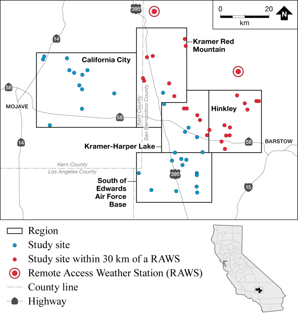
In 2021, the 55 study sites surveyed were situated in eastern Kern County and western San Bernardino County, CA, in an area extending from west of California City eastward to Hinkley Valley, and from 8 km south of Edwards Air Force Base northward to Red Mountain (Fig. 1). The geographic center of the 2021 study area was slightly east of Boron, CA, at approximately 35.001° N, –117.601° E. The sites had an elevation range of 630–1030 m. Vegetation on alluvial slopes and bajadas supported creosote bush (Larrea tridentata)-white bursage (Ambrosia dumosa) scrub, while valley floors and sinks supported saltbush scrub dominated by Mojave spinescale (Atriplex spinifera) and shadscale (At. confertifolia).

The 2020–2021 winter was exceptionally dry, with less than 30 mm of rainfall recorded at most nearby locations, representing less than 25% of the long-term average of 137 mm for the region (Hereford et al. 2003; Milbases 2024). Annual plant growth was almost lacking, and many shrubs produced very limited and sometimes early-drying foliage.

Field Methods

Study sites were grouped into five regions with 9–12 sites surveyed in each: California City; South of Edwards Air Force Base; Kramer-Harper Lake; Kramer-Red Mountain; and Hinkley. At each study site, we deployed 10 trail cameras in a 2 x 5 array with 150 m spacing. Earlier studies showed that adult female MGS often had home ranges approximately 150 m in diameter (Harris and Leitner 2004), so this spacing was intended to optimize the number of MGS potentially encountered in an area of 150 m by 600 m.

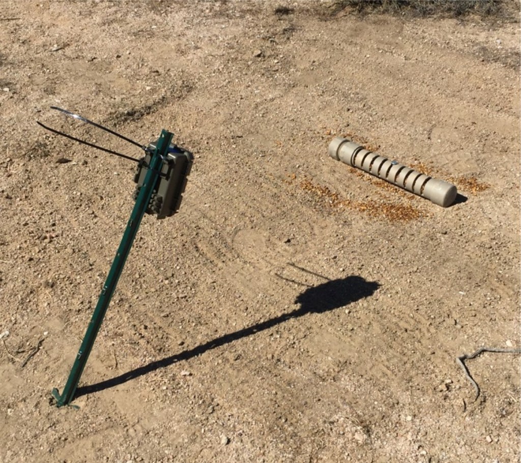
At each camera station, we cleared plant material from an area of about 1.5 m², then centered a bait tube containing attractant in the cleared area. A bait attractant is assumed to increase the likelihood of visitation by MGS, and repeated visitation results in more images, increasing the likelihood that MGS will be detected (Arvin et al. 2021). The bait tube was a 46 cm length of 5 cm diameter PVC pipe with two end caps, one fixed and one removable, 10 parallel slots each 1 cm wide and 11 cm long cut into the sides, and a 12 mm diameter hole drilled through the center of the tube. Each bait tube was filled with 0.4 kg of commercial livestock feed consisting of oats, corn, barley, and molasses, and a 3 cm diameter ball of peanut butter mixed with flour to reduce stickiness. The slots allowed animals to retrieve small amounts of bait at a time, but a little grain and all of the peanut butter ball always remained at the end of the operational period. We secured the bait tube by pounding a 30 cm long spike through the center hole in the tube and into the ground. Approximately 1 meter to the south of the tube, we set a 1 m-long metal U-post in the ground inclined slightly to the north. Using zip ties we mounted a trail camera so its field of view encompassed the bait tube and cleared area but excluded vegetation whose movement might trigger the camera (Fig. 2). We tested the camera to be sure it was properly aligned, then scattered a handful of loose mixed grain around the bait tube as an additional attractant.

We used Bushnell Trophy Cam HD trail cameras, with the following settings: daylight hours; maximum sensitivity; maximum burst of three photos per trigger event; and minimum 0.6- or 1.0-second delay between trigger events depending on the capability of the camera. At each study site we completed all camera set ups on Day 1 and operated them until Day 8. When we retrieved the cameras, we also removed the bait tube and disposed of its unused attractant off-site. On each weekday we picked up cameras from two study sites, serviced the cameras, and then set up two other study sites. We operated each camera array twice, once during Session 1, 22 February–8 April (with three study sites continuing operation until 18 April), and once during Session 2, 15 April–26 May. Due to unrelated scheduling considerations, we operated three study sites during Session 1 for 10–12 days longer, and the study site at Hinkley-7 for 12 days during Session 2. At the conclusion of the second session, we removed the cameras, tubes, spikes and U-posts.

To test the effectiveness of different attractants, we set up a randomized block design experiment during Session 2 at Hinkley-7, a study site where MGS had been detected at all camera stations during Session 1. Prior to the test, we washed the bait tubes with plain water to remove residual odors, such as from peanut butter. Within the footprint of the Session 1 150 m by 600 m camera arrangement, we centered a 5 m x 150 m array of 30 cameras in five two-by-three groups, each group separated by 25 m, and the six cameras within a group each separated by 5 m. Thus, all 30 cameras were placed in new locations well within the footprint of the Session 1 layout, and thus likely within the range of the MGS that visited the cameras during Session 1. Each group contained the following attractant combinations: 1) mixed grain in tube only; 2) peanut butter in tube only; 3) mixed grain in tube and peanut butter in tube; 4) mixed grain in tube and scattered mixed grain; 5) mixed grain in tube, peanut butter in tube, and scattered mixed grain; and 6) control, an empty bait tube. We set up the cameras and bait attractant as in the main study and operated them for 12 consecutive days.

Data Management and Analysis

After we retrieved cameras from the field, we copied data from the secure digital (SD) cards onto two duplicate hard drives to minimize risk of data loss. We examined all images, recording the vertebrate species encountered on each day of camera operation. For MGS, we counted an independent detection event as one or more MGS images separated from prior and subsequent MGS images by 30 minutes or more. We recorded the date, start, and stop time of each detection. The term “first detection” refers to the first time any MGS is detected at an individual camera, not the first time an individual MGS was detected.

As a quality control measure, we checked the accuracy of recorded MGS detections by a second observer re-examining images from 5% of randomly selected camera deployments at each study site. We corrected all errors, consisting of missed detections or incorrectly combined detections. If the error rate in this subsample was < 2%, we considered the data to be sufficiently accurate and carried out no further checking.

To evaluate the utility of the 30-minute independence interval for characterizing MGS activity patterns, we selected a study site with a large number of MGS detections, well-distributed among cameras and sessions, to maximize the potential number of individual MGS and minimize variation in environmental conditions, factors that might affect MGS behavior around a bait attractant. From Kramer-Red Mountain Site B-1 we selected 110 detections, half from each session. Using this data set we re-examined the data, varying the independence interval from 30 minutes by 1-minute increments down to one minute, recording the duration of each. In addition, we counted the number of frames in each of the 502 detections resulting from the 1-minute independence interval.

To analyze the daily activity of MGS over the period of camera deployment, we noted the first MGS detection at each camera, as well as the first detection for each day of camera operation, at all cameras during each session. We also indexed all detections against times of sunrise and sunset using data from Ridgecrest, CA, the longitudinal center of the study area (Sunrise-Sunset.org 2024). Based on longitude, all study sites deviated by < 3 minutes from the official daily sunrise and sunset times at Ridgecrest. Ignoring daylight savings time adjustment, sunrise time varied by about 50 minutes from the beginning to the end of the survey period (22 Feb–26 May 2021). We then analyzed the timing of all detections and first and last daily detections in relation to sunrise and sunset.

To compare MGS activity with that of the abundant white-tailed antelope ground squirrel (Ammospermophilus leucurus; AGS), we also randomly selected 624 camera-days with high numbers of images and AGS detections. From these camera-days, we recorded the onset time of each first daily AGS detection and the conclusion time of each last daily AGS detection.

To analyze MGS activity in relation to ambient temperature, we compared detections against camera-recorded temperature and nearby weather station data. First, we identified the two nearest Remote Automatic Weather Stations (RAWS), Opal Mountain and Red Mountain, situated 52 km apart (Desert Research Institute 2024a,b) and obtained hourly air temperature data for days when nearby camera sites were operational. Then we selected one study site, Kramer-Harper Lake-3 (KHL-3), near both weather stations (25 and 37 km from Opal Mountain and Red Mountain, respectively), and which had many images, and thus many temperature records, which are recorded with each image. From KHL-3 we recorded and averaged hourly temperatures from the 10 cameras as data were available.

The air temperatures at these two RAWS stations were in close agreement over this fairly large distance, typically differing by a degree or two, with the Opal Mountain RAWS usually having slightly higher daytime maxima. Because the RAWS stations differed by 110 m in elevation, the dry adiabatic lapse rate of 1^º C per 100 m elevation (NWS 2024) accounted for this difference. Since the Red Mountain RAWS is 330 m higher than KHL-3, we applied the dry adiabatic lapse rate adjustment and added 3.3^° C to the Red Mountain RAWS temperatures to calculate hourly estimated local shaded air temperature at KHL-3. We then compared the two RAWS hourly temperatures, the adjusted estimated air temperature for KHL-3, and the temperatures recorded by cameras at KHL-3.

Concluding that the RAWS data were a reasonable basis for estimating air temperatures at nearby study sites, we expanded our analysis of temperature and MGS activity to detection data from the 25 study sites within 30 km of either station (Fig. 1). We averaged the elevation of the study sites, 739 m, and used the adiabatic lapse rate adjustment from the RAWS data to create an estimated average air temperature for these study sites. To improve comparability of temperatures, we excluded from further consideration the three study sites more than 100 m elevation higher or lower than the average. We then tabulated the number of MGS detections, by hour; detections spanning two or more hours would be counted in each. We defined average “daytime” temperatures as the mean of hourly temperatures between 0800–1600 hrs, the period of greatest MGS activity. To compare MGS activity on warm versus cool days, we selected pairs of consecutive days with at least 4°C differences in average daytime temperature, including only data from study sites less than 30 km from either RAWS station and only pairs of days when cameras were operational for the full day; i.e., operational days 2 through 7.

For the bait attractant test, we counted all of the images in which MGS appeared for each day and each camera, and tabulated them by treatment. We used one-way ANOVA to compare all treatments and Tukey’s test to compare pairs of treatments using P < 0.05 as the critical value.

Results

Overview of 2021 Camera Study

We captured 2.65 million images in 2021, divided about evenly between the first and second sessions (1.33 M vs 1.32 M, respectively). The vast majority of images were of vertebrates, although some images contained only insects or vegetation moved by the wind. The most frequently-appearing wildlife species was the AGS, followed by the common raven, then MGS. Thirty-one other vertebrate taxa were also recorded (Leitner and Leitner 2022). Mohave ground squirrels were detected at 214 of the 550 cameras, and at 36 of the 55 study sites. Based on our definition of detection independence, we recorded a total of 2,618 MGS detections during the regular 8-day operational periods during the two sessions, with slightly more detections in Session 2 (1,474) compared with Session 1 (1,144). As is typical in unusually dry years, MGS did not reproduce in 2021; thus, the higher level of activity in Session 2 was attributable only to visitation by adults and not juvenile recruitment.

Assessment of Detection Methodology

The quality check of detection data showed that the rate of missed, or incorrectly combined detections was less than 1.6%; with this low error rate, we concluded that no further review was required for quality control.

Most MGS detections lasting longer than a minute did not contain continuous images of MGS; instead, they consisted of MGS appearing and then departing, sometimes many times, within a given detection. In varying the independence interval between detections from 30 minutes to 1 minute, the number of detections increased as the separation interval decreased, from 110 detections to 502 detections, respectively (Fig. 3). In the 502 detections resulting from the 1-minute independence interval, the median duration of a detection was 16 seconds, and the mean number of images was five per detection. Thus, the number of detections was highly dependent on the independence interval.

Patterns of MGS Detections within the Operational Period

In Session 1, the number of cameras with first detections was highest on Day 2 (26%; Fig. 4). Substantial numbers of first-time detections at new cameras continued through Day 5; one first-time detection was even recorded at a new camera on Day 8, the day cameras were removed. The average duration of detections was highest on Day 1, but the number of detections peaked on Day 6 during Session 1.

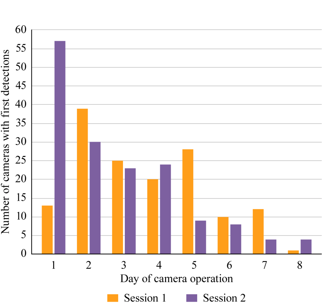
As might be expected when animals are familiar with an attractant, first detections during Session 2 took place comparatively earlier, with the number of cameras first recording MGS highest on Day 1 (36%; Fig. 4). Although first detections decreased rapidly after Day 1, they continued to be recorded on every day of camera operation, including four on Day 8 (1%). As in Session 1, the average duration of detections was highest on Day 1, but the number of detections was greatest on days 2 and 4 in Session 2.

Due to external scheduling considerations, three study sites were operated for 17, 18 and 20 days, respectively, during Session 1. In this small sample of 30 cameras, the first detections were recorded at two additional cameras after the usual 8-day operational period (days 10 and 11). These data show that MGS continue to make appearances at new cameras for a long period of time.

Patterns of Daily Activity: Time of First and Last Squirrel Detections

Timing of first and last daily detection gives an indication of when MGS are actively foraging. Overall, 99% of all MGS detections began at least 2 hours after sunrise (Table 1). The highest levels of activity were recorded during midday, from 5 to 11 hours after sunrise. This pattern was consistent throughout the three-month survey period.

Table 1. Onset of all Mohave ground squirrel detections, in hours after sunrise, 2021.

Hours after Sunrise	Detectionsa	% of Total	Cumulative %
0–1	2	0%	0%
1–2	28	1%	1%
2–3	150	6%	7%
3–4	231	9%	16%
4–5	238	9%	25%
5–6	261	10%	35%
6–7	283	11%	46%
7–8	255	10%	56%
8–9	282	11%	67%
9–10	304	12%	79%
10–11	255	10%	88%
11+	324	12%	100%
Total	2,613	100%	—

MGS detections generally ended well before sunset (Table 2). About 88% of MGS detections concluded by at least 2 hours before sunset, and only 2% extended into the last hour before sunset. This pattern of late afternoon activity was similar throughout the three-month survey period.

Table 2. Conclusion of all Mohave ground squirrel detections, in hours before sunset, 2021.

Hours before Sunset	Detectionsa	% of Total	Cumulative %
11+	65	2%	2%
10–11	134	5%	8%
9–10	191	7%	15%
8–9	257	10%	25%
7–8	262	10%	35%
6–7	247	9%	44%
5–6	273	10%	55%
4–5	273	10%	65%
3–4	296	11%	76%
2–3	299	11%	88%
1–2	257	10%	98%
0–1	59	2%	100%
Total	2,613	100%	—

In contrast to MGS, AGS were usually the first diurnal vertebrate species to appear in the morning, and the last to be recorded before sunset (see Supplemental Information Tables S1 and S2). Whereas only 2.5% of MGS first daily detections began within two hours after sunrise (Table 1), 68% of AGS first daily detections had already begun by this time. At the end of the day, almost one-quarter of AGS detections extended into the last two hours before sunset, twice the proportion of MGS. Thus, AGS have a much longer period of daily activity, beginning near sunrise and extending to near sunset, while MGS have a shorter period of daily activity centered on early afternoon.

Although the cameras were set for daytime operation, they actually recorded images as early as 20 minutes before the official sunrise at Ridgecrest. Images recorded pre-sunrise were almost exclusively of nocturnal kangaroo rats (Dipodomys spp.), although pocket mice (Perognathus spp. and Chaetodipus spp.), common ravens, and desert kit fox (Vulpes macrotis arsipis) were also recorded. Typically, an hour or more passed between the before-sunrise photos recorded and the first appearance of diurnal animals such as AGS. The earliest MGS detection was recorded 34 minutes after sunrise.

MGS Activity in Relation to High Temperature

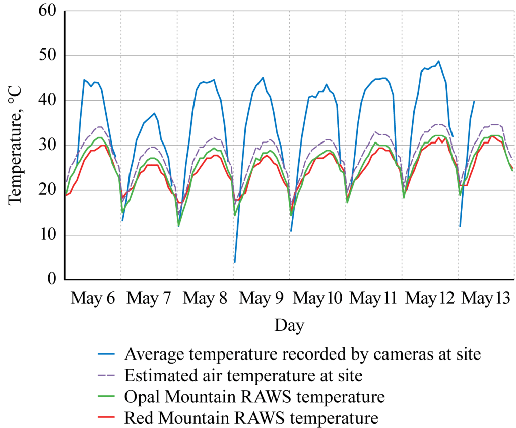
Estimating air temperature.—In comparing the average hourly temperature curve recorded by cameras at the KHL-3 site, the two nearby RAWS sites, and the calculated estimated site air temperature at KHL-3, we found that the average temperature recorded by the cameras at KHL-3 rose 8–15^° C higher than the calculated estimated site air temperature (Fig. 5). Low temperatures recorded by the cameras at sunrise often were lower than the air temperature recorded at the RAWS sites, as would be expected due to nighttime energy radiation. These data demonstrated that temperatures recorded by our unsheltered cameras are too variable to represent shaded air temperature, but that nearby RAWS data may be adjusted to approximate local temperatures at nearby study sites based on elevation. These estimated temperatures will be used in the analyses that follow.

Patterns of MGS activity in relation to high temperature.—During the five warmest days of the survey period, all during Session 2, MGS detections were most numerous in the warmest part of the day (Table 3). On 30 April, the warmest day in our study period, 70% of all MGS detections took place when estimated shaded air temperatures exceeded 32°C. On other days this proportion ranged from 34–67%, the lower proportions likely related to the briefer periods of warmer temperatures. This shows that MGS foraging activity, as indicated by detections, remained high, or even peaked during warm periods, at least during the temperatures prevailing during the survey period.

Table 3. Number of Mohave ground squirrel detections and estimated temperature, by hour, during warmest five days of survey, 2021.

Table 3a. 30 April 2021

Time	Air Tempa (ºC)	Detections	% Detections when T > 32° C
0600	23.3	2	—
0700	24.4	5	—
0800	27.2	10	—
0900	29.4	10	—
1000	31.6	11	—
1100	33.9	11	9%
1200	34.4	7	6%
1300	35.0	9	8%
1400	35.0	14	12%
1500	35.5	14	12%
1600	35.0	18	15%
1700	34.4	7	6%
1800	32.2	2	2%
Total	—	120	70%

Table 3b. 12 May 2021

Time	Air Tempa (ºC)	Detections	% Detections when T > 32° C
0600	24.4	2	—
0700	25.5	5	—
0800	27.8	6	—
0900	29.4	8	—
1000	31.6	6	—
1100	32.8	6	10%
1200	32.8	5	8%
1300	33.9	4	6%
1400	34.4	6	10%
1500	34.4	6	10%
1600	34.4	5	8%
1700	33.9	3	5%
1800	32.2	0	0%
Total	—	62	57%

Table 3c. 13 May 2021

Time	Air Tempa (ºC)	Detections	% Detections when T > 32° C
0600	23.9	2	—
0700	25.0	2	—
0800	27.8	6	—
0900	30.0	3	—
1000	31.1	3	—
1100	32.8	4	8%
1200	33.9	4	8%
1300	33.9	3	6%
1400	34.4	5	9%
1500	34.4	6	11%
1600	34.4	9	17%
1700	33.9	4	8%
1800	30.5	2	—
Total	—	53	67%

Table 3d. 14 May 2021

Time	Air Tempa (ºC)	Detections	% Detections when T > 32° C
0600	22.8	0	—
0700	25.5	3	—
0800	27.2	5	—
0900	28.9	8	—
1000	30.0	5	—
1100	31.6	6	—
1200	32.8	4	8%
1300	32.9	2	4%
1400	33.9	6	12%
1500	33.9	4	8%
1600	33.3	4	8%
1700	31.6	2	—
1800	28.9	1	—
Total	—	50	40%

Table 3e. 18 May 2021

Time	Air Tempa (ºC)	Detections	% Detections when T > 32° C
0600	18.9	3	—
0700	22.2	6	—
0800	24.4	3	—
0900	27.2	6	—
1000	29.4	5	—
1100	31.1	6	—
1200	33.3	2	4%
1300	33.9	2	4%
1400	33.9	2	4%
1500	33.3	5	10%
1600	33.3	6	12%
1700	31.6	4	—
1800	27.8	1	—
Total	—	51	34%

We also examined MGS detections during the warmest five days of Session 1, which encompassed 8 March–8 April for the 25 study sites within 30 m of the Red Mountain and Opal Mountain RAWS. The five highest daily temperature maxima occurred on 28 and 29 March and 2–4 April, which ranged from 26.6–30.5°C. The number of MGS detections on these relatively mild temperature days was so small (n = 51) that no pattern of MGS activity could be discerned in relation to hourly temperature.

MGS Activity in Relation to Low Temperature

We examined relative MGS activity on successive days with high and low temperatures to see if daily temperatures influenced number of detections. Out of the seven pairs of days when the first day daytime average was at least 4°C cooler than the second day, in six instances the number of MGS detections was higher on the warmer, second day, sometimes considerably so (Table 4). For example, March 15 was the coolest such day at 8.9°C; the next day was 5.3°C warmer. The first and second days had 10 and 43 MGS detections, respectively. The effect of increased MGS foraging activity on a warmer day following a cool day was more pronounced during Session 1 when overall temperatures were relatively low. When both days were relatively warm, as in Session 2, the difference in between detected activity between days was negligible.

In the eight pairs of days with the mean daytime temperature of the first day at least 4°C warmer than the second day, MGS detections were more numerous in six of the warmer days (Table 5). In these examples MGS detections averaged 57% more on the warmer day compared with the second, cooler, day. Again, the greater contrast between days was during Session 1 when prevailing temperatures were cooler overall.

Table 4. Number of Mohave ground squirrel detections on consecutive days when the estimated average daytime temperature was at least 4° C warmer on the second day, March–May 2021.

Session	Day	Date	Avg Day Temp (°C)a	# Detections
Session 1	Day 1	12 March	9.4	18
Session 1	Day 2	13 March	14.0	24
Session 1	Day 1	15 March	8.9	10
Session 1	Day 2	16 March	14.2	43
Session 1	Day 1	26 March	16.2	8
Session 1	Day 2	27 March	20.7	21
Session 1	Day 1	27 March	20.7	21
Session 1	Day 2	28 March	25.2	24
Session 2	Day 1	16 May	22.9	25
Session 2	Day 2	17 May	27.4	30
Session 2	Day 1	17 May	27.4	30
Session 2	Day 2	18 May	31.6	27
Session 2	Day 1	23 May	23.4	5
Session 2	Day 2	24 May	28.2	10

Table 5. Number of Mohave ground squirrel detections on consecutive days when the estimated average daytime temperature was at least 4°C cooler on the second day, March-May, 2021.

Session	Day	Date	Avg Day Temp (°C)a	# Detections
Session 1	Day 1	14 March	18.0	34
Session 1	Day 2	15 March	8.9	12
Session 1	Day 1	19 March	21.8	29
Session 1	Day 2	20 March	14.5	28
Session 1	Day 1	29 March	24.9	12
Session 1	Day 2	30 March	20.5	10
Session 2	Day 1	30 April	33.4	75
Session 2	Day 1	1 May	29.4	65
Session 2	Day 1	14 May	31.4	29
Session 2	Day 2	15 May	27.2	27
Session 2	Day 1	15 May	27.2	27
Session 2	Day 2	16 May	22.9	31
Session 2	Day 1	19 May	28.9	3
Session 2	Day 2	20 May	21.7	3
Session 2	Day 1	20 May	21.7	9
Session 2	Day 2	21 May	15.9	3

Bait Attractant Test

Peanut butter-only and control (empty) bait tubes comprised 33% of test attractant stations but provided only 1.6% of MGS images generated by all cameras, while test attractant stations with grain comprised 67% of stations and provided 98.4% of images (Table 6). Although this suggests that grain is an effective attractant, and certainly suggests that grain encourages repeat visitation by MGS, the large number of cameras with no MGS detections (15 out of 30) resulted in very high variance and statistical testing was problematic. Using the one-way ANOVA test, we found no significant difference between the number of frames containing MGS images at the control and the five attractant combinations (P = 0.076). Comparing individual bait attractant combinations pairwise using Tukey’s test again showed no significant difference (Table 7). The null hypothesis of no significant difference between test alternatives therefore cannot be rejected. While the summary data appear to suggest that the contribution of peanut butter in attracting MGS is minimal, a sample with smaller variance would be necessary to demonstrate this.

Table 6. Comparison of attractant combinations, by number of frames in which Mohave ground squirrels appeared. Data from Hinkley Site 7, May 13–24, 2021. No pairwise comparisons were significantly different.

Treatment: Attractant Presented	# Images Detected	% Images
Mixed grain inside tube + mixed grain scattered on ground (BS)	793	48%
Mixed grain in tube only (B)	372	22%
Mixed grain + peanut butter in tube + mixed grain scattered on ground (BPS)	304	18%
Mixed grain + peanut butter in tube (BP)	164	10%
Peanut butter in tube only (P)	25	2%
Control—empty bait tube (C)	2	<1%
Total	1,660	100%

Table 7. Pairwise comparisons of bait attractant combinations using Tukey’s test. (CI = Confidence Interval)

Attractant Comparisona	Difference in Means	Lower CI	Upper CI	P–value
BS–BPS	45.817	–6.379	98.012	0.116
BS–BP	49.683	–8.021	107.388	0.129
BS–B	39.512	–13.506	92.529	0.252
P–BS	–57.750	–144.743	29.243	0.375
C–BS	–65.083	–168.015	37.848	0.430
C–B	–25.571	–127.447	76.304	0.975
P–B	–18.238	–103.980	67.503	0.988
C–BPS	–19.267	–120.717	82.184	0.993
BP–B	–10.171	–65.971	45.628	0.994
C–BP	–15.400	–119.792	88.992	0.998
P–BPS	–11.933	–97.169	73.302	0.998
BPS–B	–6.305	–56.387	43.777	0.999
P–BP	–8.067	–96.783	80.649	0.999
BPS–BP	3.867	–51.153	58.886	0.999
P–C	7.333	–115.694	130.360	0.999

 ^a BS: Mixed grain inside tube + mixed grain scattered on ground; BPS: Mixed grain inside tube + peanut butter in tube + mixed grain scattered on ground; BP: Mixed grain inside tube + peanut butter in tube; B: Mixed grain in tube only; P: Peanut butter in tube only; C: Control—empty bait tube

Discussion

MGS Activity in Relation to Temperature

The interpretation of our results is influenced by an overarching theme: the critical importance to MGS of optimizing their energy budget during their relatively brief annual period of sustained above-ground activity from late winter to summer. During this time adults must nearly double their body weight by accumulating fat to survive their extended dormancy, as well as reproduce and rear young when conditions allow (Leitner and Leitner 2017). MGS accomplish this feat in part by physiological adaptations that allow for estivation, a wide range of non-estivating body temperature, and efficient use of water (Bartholomew and Hudson 1960, 1961). In addition, they employ behavioral adaptations that minimize energy loss during cool ambient temperatures; promote passive warming by basking under cool conditions; maximize activity when ambient temperatures demand little energy output; and dissipate excess heat when necessary.

Among sciurids, MGS have unusually labile body temperatures; in addition to dropping their body temperature to near ambient during estivation/hibernation, MGS have a broad thermal neutral zone, from 25^° to 36.7^° C (Bartholomew and Hudson 1961). Recht (1977) documented that MGS body temperatures routinely drop overnight by up to 4^° C during the MGS active season. He found that they regain their optimum active temperature through piloerection, basking and positioning perpendicular to the sun at their burrow entrances before engaging in other daily activities such as foraging. In cool temperatures during spring this process can take 80–120 minutes, but only 5–20 minutes in warm temperatures in summer. He also documented that MGS can quickly dissipate excess heat in warm weather by retreating to the shade of shrubs; transferring heat to the soil by pressing themselves onto cooler soil or into small depressions they have excavated in the shade; or by entering burrows (Recht 1977).

Consistent with these findings, nearly all MGS detections began 2 hours after sunrise during our study period and concluded at least an hour before sunset when temperatures fall. Recht (1977) found that MGS had a shorter basking period during warmer summer temperatures and thus initiate activity beyond the burrow entrance somewhat earlier. However, even in summer MGS foraging activity still began well after sunrise. As measured by detections, MGS during Session 1 were much more active on warm days compared with cooler days preceding or following. Even on the warmest days of our study in Session 2, MGS were most active during the warmest portions of the day. Shaded air temperatures during our study reached an estimated 35°C, still within the MGS thermal neutral zone. Under these conditions MGS can maintain activity with little energy expended for warmth, and can regulate their temperature by cooling off. Because our study concluded before the onset of the highest summer temperatures, our data could not confirm Recht’s (1977) finding that MGS activity diminished during the highest summer temperatures, when cooling off may be costly in terms of water loss. All of these results underscore the close energetic limits within which MGS must live, and indicates a close relationship between ambient temperature and MGS activity. The results also emphasize the need for close attention to temperature when live-trapping, because MGS are active during warm temperatures, yet they cannot employ their usual cooling behaviors when confined to a trap.

The annual period of sustained MGS activity begins in early February, when overnight freezing is frequent and daytime high temperatures may reach no more than 10^° C. Basking under these conditions would be insufficient for MGS to reach optimum body temperatures; more active and energetically costly behavioral measures would be necessary to warm up. As measured by detections, the absolute air temperatures when MGS are most active changes throughout their active season, but they typically are most active during the warmest part of the day, at least within their thermal neutral zone. While physiological flexibility helps the MGS maintain activity over a wide range of temperatures, behavioral adaptations to conserve and dissipate energy are also necessary.

Although our analysis showed that air temperature can reasonably be estimated over a large area using existing data sets and adjusting for elevation, temperature can also be influenced by other factors, such as prevailing winds, topography, and air circulation patterns. An on-site weather station is the most accurate measure of local air temperature.

Although camera-recorded temperature is much more variable than air temperature, it also is an indication of an important element of the thermal environment experienced by MGS (Bakken 1992), that of unshaded temperatures. MGS do most of their foraging on the ground, and in high temperatures they must traverse open soil with temperatures that may resemble that recorded by the cameras. We found the maximum daily temperature differential between camera-recorded temperature and estimated site shaded air temperature averaged 12.6^° C during 6–13 May (Fig. 5), while Recht (1977) found a measured maximum differential between soil surface and air temperatures of 12^° C in July. Thus, camera-recorded temperature can serve as an approximation for soil temperature.

Further, Recht (1977) found a maximum daily difference of more than 20° C between soil surface in the sun and in the shade. He described a characteristic heat-dissipating behavior of MGS in which animals press their bodies into the cooler, shaded soil, directly transferring heat from their bodies to the soil. One physical adaptation for MGS travel on hot soil includes densely-haired soles on the hind feet (Best 1995). The substantial difference between air temperature and sun and shade soil surface temperatures underscores the importance of shaded soil for MGS cooling behaviors.

An Analysis of Study Methods

Although we do not usually see quality control methods described for camera studies, we found the practice useful. Reviewing camera data, in our case 2.5 M images in 2021, is a lengthy process and requires sustained attention. In conducting a quality check, we found that one reviewer had more errors than the other reviewers combined. Our solution was to re-review and correct all of that reviewer’s work. Without quality control, those errors would have been missed. We conclude that the best quality control procedure is for investigators to review small portions of each other’s work regularly during the reviewing period to identify systematic errors and reinforce practices such as taking breaks to avoid diminished concentration.

We initiated the use of independence intervals and detections as an effort to quantify MGS activity beyond presence-absence without resorting to the onerous task of counting MGS frames in our large data set. The independence interval selected, 30 minutes, was arbitrary (Kays et al. 2016), so we investigated whether a shorter interval would be more meaningful in terms of MGS behavior. We expected to find a break in slope in Fig. 3 if there were a behavioral basis for independence intervals of 1–30 minutes, but we found none. Continuous MGS appearances at a camera (i.e., successive images containing the same individual MGS, based on appearance and positioning) usually was quite brief, typically only a few seconds. Longer detections were characterized by MGS departing and returning to the camera, sometimes many times. Thus, we found no basis for any particular independence interval and conclude that any independence interval would be arbitrary and not based on MGS behavior.

Protocol for MGS camera trapping strongly recommends a minimum of three 5-day camera deployments (CDFW 2023), in conjunction with live-trapping. The 8-day deployment period in this study provided an opportunity to assess whether longer operating periods could significantly increase the probability of detecting MGS. If hypothetical 5-day deployments had begun at the same time as ours and ended at 1600 hours on Day 5 throughout our study period, 10.5% fewer cameras would have detected MGS and the number of study sites with MGS detections would have been 35 instead of 36.

A review of the camera settings and timing of images showed that daytime settings are adequate for detecting MGS. Although the cameras in this study were set for daylight hours, the cameras actually recorded other species up to 20 minutes before the official sunrise time at Ridgecrest. This was nearly an hour earlier than the earliest morning MGS record—34 minutes after sunrise—demonstrating that daytime camera settings were sufficient to record the earliest daily MGS activity.

Meek et al. (2014) noted that camera trap performance is affected by weather, particularly extreme heat and cold, due to the sensitivity of their passive infra-red sensors, and that sensors may become less reliable as the temperature differential decreases between the moving object and ambient. In our study, the highest temperature recorded by the cameras was 49°C when the corresponding estimated air temperature was 35° C.Both are at or above the normal MGS body temperature of 35.8°C (Recht 1977; Best 1995). In our experimental design of placing a bait attractant 2 m or less from the camera, MGS are large enough to effectively trigger the camera, at least during the moderately warm temperatures prevailing during April and May.

The continued activity of MGS at cameras throughout the 8-day deployment period demonstrated that the bait tube presentation continued to be attractive to MGS for at least a week. The test of bait attractant did not show significant differences between test elements at the P < 0.05 level. However, the raw data suggest that mixed grain, whether scattered loosely or within a bait tube, is an effective attractant, while peanut butter presented alone received few visits. Further investigation resulting in a larger sample size with less variance would be needed to ascertain if differences between bait attractant alternatives are statistically significant or not.

In general, the mixed grain offers a food reward while the peanut butter within the tube was never consumed, even partially. Use of a bait tube provides less food subsidy for common ravens and eliminates the need to service the bait attractant during the operational period of the cameras, apparently remaining attractive to MGS for at least one week. Compared with live-trapping, cameras can be deployed with less effort for full days, for longer periods and under all weather conditions with less risk to wildlife. Thus, baited cameras serve as a valuable tool for investigating the presence of MGS.

Camera Results in Relation to Squirrel Behavior

The probability of MGS detection at a given camera depends on a variety of factors—the number and spacing of cameras; length of deployment; attractant, if any; and external factors, such as the availability of other types of forage, proximity to MGS burrows, number of MGS present, nutritional and reproductive status of MGS, especially juvenile recruitment; and camera placement in relation to MGS home ranges and travel routes. Recht (1977) found that his radiocollared MGS utilized a network of runways and that most of their activity took place within 30 cm of these runways, which he estimated at less than 3% of the area within their home range polygons.

The element of chance as to whether an MGS encounters a camera and attractant is also illustrated by the pattern of MGS detections in the bait attractant test. There, 30 cameras were situated in an area 5 m by 150 m, the same length as the distance between just two cameras in our typical array, yet in 12 days of deployment only about half the stations yielded detections, even among those with grain attractant, which is widely held to be an effective bait.

It would be highly desirable to be able to reliably index the number of detections or images to the number of individual MGS present, or to estimate population size. At present, we do not have a method to do this. As discussed in the preceding section, many factors affect the likelihood of an MGS being detected by a camera. Although our cameras were spaced well apart based on a typical MGS home range, home range size can vary considerably within the MGS active period, and from year to year based on food availability, among other factors (Harris and Leitner 2004). Another confounding factor is that of juvenile recruitment and dispersal. Reproduction occurs among MGS in some but not all years, so populations can vary considerably in numbers and areal extent, especially during a series of consecutive reproductive or non-reproductive years. And when reproduction is successful, juveniles disperse widely, resulting in detections in a larger area where MGS may not be permanent residents.

Although some investigators can reliably distinguish individual MGS in camera studies, we could not, unless they had distinguishing molt patterns, injuries, or other distinctive features. Still, among individual MGS that could be distinguished, we noted that in 2021, a year with very low food availability, these individuals sometimes visited up to four camera stations, suggesting that their home range was larger than the average 150 m diameter home range calculated for adult female MGS by Harris and Leitner (2004). If detections or images cannot provide an index to number of individuals or population estimate, there is little reason to analyze camera data at this level for ordinary protocol surveys, although such granular data can provide the basis for other investigations such as the temperature and temporal analysis presented here.

Currently, the most comparable metric across investigations is simply presence or absence of MGS. We hope that this study, together with others, can support the development of standardized camera trapping field and analytical methods. This will help to develop a greater level of comparability between investigations, even if an index of MGS abundance remains elusive.

Acknowledgments

We gratefully acknowledge the following individuals and organizations: foremost, M. Recht, for his careful observations of MGS that informed the interpretation of our data and for his review of the manuscript; J. Hopkins, who fostered our early studies of this species; A. Baker, Habitat Conservation Planning Branch, CDFW, who assisted us with statistical analysis; A. Fesnock, BLM, for envisioning this study and securing funding; Conservation Global International, for project management; our field crew, K. Tabor, M. Gaytan, S. Garcia, A. Gil, and A. Ruvalcaba; and anonymous reviewers who provided helpful input. This project was funded by the U.S. Bureau of Land Management, California State Office, Sacramento, CA.

Literature Cited

• Arvin, A. C., C. E. Pekins, J. H. Sperry, and M. L. Allen. 2011. Evaluating the efficacy and decay of lures for improving carnivore detections with camera traps. Ecosphere 12(8). https://doi.org/10.1002/ecs2.3710
• Bakken, G. S. 1992. Measurement and application of operative and standard operative temperatures in ecology. American Zoologist 32:194–216.
• Bartholomew, G. A., and J. W. Hudson. 1960. Aestivation in the Mohave ground squirrel, Citellus mohavensis. Bulletin of the Museum of Comparative Zoology, Harvard 124:193–208.
• Bartholomew, G. A., and J. W. Hudson. 1961. Desert ground squirrels. Scientific American 205:107–116.
• Best, T. L. 1995. Mojave ground squirrel Spermophilus mohavensis. Mammalian Species 509:1–7.
• California Department of Fish and Wildlife (CDFW). 2023. California Department of Fish and Wildlife Mohave Ground Squirrel Survey Guidelines. October 2023 revision. California Department of Fish and Wildlife, Sacramento, CA, USA.
• Desert Research Institute University of Nevada Reno. 2024a. Station Monthly Summary, Opal Mountain, CA, USA. Available from: https://wrcc.dri.edu/cgi-bin/rawMAIN.pl?caCOPA (Accessed: 22 February 2024)
• Desert Research Institute University of Nevada Reno. 2024b. Station Monthly Summary, Red Mountain, CA, USA. Available from: https://wrcc.dri.edu/cgi-bin/rawMAIN.pl?caCSQS (Accessed: 22 February 2024)
• Harris, J. H., and P. Leitner. 2004. Home-range size and use of space by adult Mohave ground squirrels, Spermophilus mohavensis. Journal of Mammalogy 85(3):517–523.
• Hereford, R., R. H. Webb, and C. I. Longpre. 2003. Precipitation History of the Mojave Desert Region, 1893–2001. Available from: https://pubs.usgs.gov/fs/fs117-03/ (Accessed: 24 February 2024)
• Kays, R., A. W. Parsons, M. C. Baker, E. L. Kailes, T. Forrester, R. Costello, C. T. Rota, J. J. Millspaugh, and W. J. McShea. 2016. Does hunting or hiking affect wildlife communities in protected areas? Journal of Applied Ecology 54:242–252.
• Langlois, N. A., T. L. Franklin, L. M. Conner, and G. Morris. 2024. Mitigating heat exposure inside Sherman traps: efficacies of various techniques. Southwestern Naturalist 23(2):162–174. https://doi.org/10.1656/058.023.0203
• Leitner, B. M., and P. Leitner 2017. Diet of the Mohave ground squirrel (Xerospermophilus mohavensis) in relation to season and rainfall. Western North American Naturalist 77(1):1–13.
• Leitner, P. 2021. Current status of the Mohave ground squirrel: an update covering the period 2013–2020. California Fish and Wildlife Journal Special, CESA Special Issue 300–316. www.doi.org/10.51492/cfwj.cesasi.18
• Leitner, P., and D. K. Delaney. 2014. Mohave ground squirrel camera study 2011–2012. Final report to California Department of Fish and Wildlife, Sacramento, CA, USA.
• Leitner, P., and B. M. Leitner. 2022. Mohave ground squirrel camera study 2021–2022. Prepared for U.S. Bureau of Land Management, Sacramento, CA, USA.
• Meek, P. D., G. Ballard, A. Claridge, R. Kays, K. Moseby, T. O’Brien, A. O’Connell, J. Sanderson, D. E. Swann, M. Tobler, and S. Townsend. 2014. Recommended guiding principles for reporting on camera trapping research. Biodiversity Conservation 23:2321–2343. www.doi.org/10.1007/s10531-014-0712-8
• Milbases. 2024. Weather & Climate at Edwards Air Force Base in Edwards, CA.Available from: https://www.milbases.com/california/edwards-air-force-base/weather (Accessed February 24 2024)
• National Weather Service (NWS). 2024. Dry adiabatic lapse rate. Available from: https://forecast.weather.gov/glossary (Accessed 22 February 2024)
• Recht, M. A. 1977. The biology of the Mohave ground squirrel, Spermophilus mohavensis: home range, daily activity, foraging and weight gain and thermoregulatory behavior. Dissertation, University of California, Los Angeles, CA USA.
• Sunrise-Sunset.org. 2024. Sunrise and sunset at Ridgecrest, CA, 2021. Available from: https://sunrise-sunset.org/us/ridgecrest-ca (Accessed: 22 February 2024)