Aspects of the population ecology of western Joshua tree in the western Antelope Valley, Mojave Desert, California

MONOGRAPH

Michael D. White¹*, Laura Pavliscak², and Mitchell Coleman¹

¹ Tejon Ranch Conservancy, 1601 New Stine Road #185, Bakersfield, CA 93309, USA
https://orcid.org/0000-0001-7153-3128 (MDW)
² Ventura Land Trust, 353 Sanjon Road,  Ventura, CA 93001, USA

*Corresponding Author: mwhite@tejonconservancy.org

Published 22 May 2026 • doi.org/10.51492/cfwj.112.3

Abstract

We examined the population ecology of western Joshua trees (Yucca brevifolia) in the Antelope Valley of the western Mojave Desert, California. The western Joshua tree is an iconic species of the Mojave Desert and a species of conservation concern in California. The Antelope Valley supports extensive, unstudied stands of Joshua tree, which are biogeographically unique and morphologically distinct from other stands across its range. In this region, largely clonal stands of western Joshua tree occur at the western leading edge of its range, where the Mojave Desert meets the Tehachapi Mountains, southern Sierra Nevada, and Transverse Ranges. Climate regimes here differ markedly from those in the rest of the range. Patchily distributed stands of dense, short-statured Joshua tree stems dominate our study area on the bajadas, washes, and canyons of the Tehachapi Mountains. The proportion of stems representing unique genets remains unclear. From 2010 to 2023, a span of 13 years, we monitored growth rates and changes of number of apical growth points of several hundred individually marked Joshua tree stems within 23 plots. Stem densities of clonal populations were an order of magnitude higher than the maximum densities reported from non-clonal populations. The high survival and growth rates of these stems were comparable to rates reported in other parts of its range, but height and number of branches are lower than in non-clonal populations. While fire is considered to play a driving role in the development of the clonal growth form, we documented significant rhizomatous stem production and high rates of height and branch regression in the absence of fire. We hypothesize that stem height and branch regression in this landscape are due to damage from high winds, which may also play a role in shaping stand architecture by pruning stems. In Joshua tree stands subject to significant wind damage, estimating age from stem height and mean growth rates become more uncertain. Production and survival of clonal stems is dynamic, and stem densities and stand architecture can change rapidly.

Key words: Antelope Valley, branch regression, clonal reproduction, growth, Joshua tree, stem height, survival, Yucca brevifolia

Citation: White, M. D., L. Pavliscak, and M. Coleman. 2026. Aspects of the population ecology of western Joshua tree in the western Antelope Valley, Mojave Desert, California. California Fish and Wildlife Journal 112:e3.

Editor: Cherilyn Burton, Habitat Conservation Planning Branch

Submitted: 8 October 2025; Accepted: 7 January 2026

Copyright: ©2026, White et al. This is an open access article and is considered public domain. Users have the right to read, download, copy, distribute, print, search, or link to the full texts of articles in this journal, crawl them for indexing, pass them as data to software, or use them for any other lawful purpose, provided the authors and the California Department of Fish and Wildlife are acknowledged.

Funding: The Tejon Ranch Conservancy provided funding for this research.

Competing Interests: The authors have not declared any competing interests.

Introduction

The western Joshua tree (Yucca brevifolia) is an iconic species of the Mojave Desert (Fig. 1) and a species of conservation concern in California (CDFW 2025). Y. brevifolia is threatened by climate change, increased fire frequency and intensity, and habitat loss (Cole et al. 2011; Barrows and Murphy-Mariscal 2012; Wilkening et al. 2020; CDFW 2022, 2025; USFWS 2023a,b; Shryock et al. 2025). To provide for its protection and long-term management, the California Legislature enacted the Western Joshua Tree Conservation Act (State of California 2023), and the California Department of Fish and Wildlife prepared a Western Joshua Tree Conservation Plan (CDFW 2025). However, little ecological research has been conducted in the Antelope Valley to inform Y. brevifolia conservation and management. The objective of our study was to measure baseline ecological characteristics of the dense, short-statured Y. brevifolia stands present on the property for which we have management responsibility and that are widely distributed in other areas of the western Mojave Desert. This research increases our quantitative understanding of the population characteristics of Y. brevifolia exhibiting a unique growth habit in a virtually unstudied region.

The taxonomy, general distribution, and ecology of Y. brevifolia are described in detail by Lenz (2007), Royer et al. (2016), and Esque et al. (2023), with recent reviews by Wilkening et al. (2020), the California Department of Fish and Wildlife (2022), and the U.S. Fish and Wildlife Service (2023b). Y. brevifolia occurs across California and Nevada, while the closely related eastern Joshua tree (Y. jaegeriana) ranges to its east (Fig. 1). Seedling establishment is rare (Webber 1953; Comanor and Clark 2000; Esque et al. 2015), but new stems can also be produced asexually from rhizomes (Simpson 1975; Comanor and Clark 2000; DeFalco et al. 2010), and dense stands of low-statured stems derived primarily from rhizomes occur along the western margin of its range (Webber 1953). Resprouting following fire is considered an adaptation of Y. brevifolia to fire disturbance (Loik et al. 2000; Gucker 2006; DeFalco et al. 2010) and fire is thought to be a driving factor producing the rhizomatous growth form (Keeler-Wolf 2007). Branching is pseudodichotomous (Simpson 1975). Leaves grow in clusters from apical growth points until growth is interrupted by the development of an inflorescence or damage to the apical growth point. Death of a growth point is followed by two to three dormant buds initiating growth and ultimately developing into new branches, so the number of branches on a stem is related to the number of times it has flowered (McKelvey 1938; Simpson 1975).

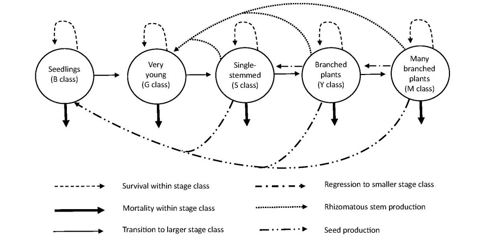
Y. brevifolia does not form annual growth rings (Simpson 1975), making it difficult to age individuals directly. Comanor and Clark (2000) proposed five age-form classes (Table 1; Fig. 2a–e). We expanded these into a stage class model for our study population (Fig. 3), where S, Y, and M class stems can flower and produce seeds as well as grow rhizomes that can produce G class stems. Stems grow and transition between stage classes (e.g., S class to Y class) or regress a stage class because of loss of branches from damage (e.g., M class to Y class). We use this model to structure our analysis and discussion.

Table 1. Age-form classes (Comanor and Clark 2000) used in this study.

Stage class	Description
B	Seedlings with slender, grass-like leaves
G	Very young plants with fleshy leaves and no stem
S	Visible stem with a single growth point
Y	Post-reproductive plant with two to nine growth points
M	Mature stem with 10 or more growth points

Methods

 Study Area

Our study area (Fig. 1) was located on the privately owned Tejon Ranch (34.889º, –118.580º) on the southern flank of the Tehachapi Mountains in the western Antelope Valley of the Mojave Desert of California (i.e., within the High Desert Plains and Hills Subsection of the Mojave Desert Section of the American Semi-Desert and Desert Province; Cleland et al. 2007). Stands of Y. brevifolia in the study area appear qualitatively different in density and stature from populations in other parts of its range, and are characterized by patches of low stature, densely clumped stems (Fig. 2f). All Y. brevifolia on the property is on land permanently conserved under the 2008 Tejon Ranch Conservation and Land Use Agreement (Reynolds and Nagami 2011; White et al. 2011; White and Penrod 2012), and our study plots are >7 km from non-conserved areas of Tejon Ranch.

The Antelope Valley (Fig. 4) extends eastward from the intersection of the Transverse Ranges and Tehachapi Mountains and drains internally to Rosamond and Rodgers Dry Lakes (CRWQCB 2021). This portion of the Mojave Desert ecoregion within the Desert Province lies at the ecotone with the Western Transverse Ranges and Tehachapi subecoregions within the California Floristic Province (Baldwin et al. 2012). The 1991–2020 climate normals for the Antelope Valley show average annual total precipitation of 120–160 mm in the valley floor and 200–350 mm in the foothills, but summer precipitation (Jul–Sept) averaged <10 mm/yr. Average daily maximum temperatures on the valley floor were 36–38ºC and 33–35ºC in the foothills and average daily minimum temperature on the valley floor was –1.6–0ºC and 0.3–2.5ºC in the foothills (PRISM Climate Group 2021). There are no contemporary records of wildfire in our study area (CAL FIRE 2025).

Our study landscape is comprised of broad middle- to late-Pleistocene alluvial terraces at the base of the southeast-facing Tehachapi Mountain escarpment dissected by drainages carrying Quaternary alluvium (Dibblee 1963, 2008). At the mouths of the larger canyons cutting through these terraces are large fans of Quaternary alluvium forming bajadas that rim the valley floor. The most extensive and dense stands of Y. brevifolia in our study area grow in alluvial soils (Hanford and Oak Glen) within washes and canyon bottoms, adjacent toes of slopes, and on the large alluvial fans at the mouths of these canyons (Fig. 5). Manual of California Vegetation (Sawyer et al. 2009) types include Joshua tree woodland, California buckwheat scrub, rubber rabbitbrush scrub, Mormon tea scrub, California juniper woodland, and desert needlegrass grassland (CDFW 2015, 2021, 2024). Stands of Y. brevifolia also occur on scattered foothill knolls between the canyons, where vegetation is mapped as California juniper woodland and California buckwheat scrub (CDFW 2015, 2021, 2024). At its highest elevations in this landscape, Y. brevifolia stems extend up into lower-elevation piñon pine (Pinus monophylla) forests (not mapped). Y. brevifolia stands qualitatively similar to those in our study area continuing off the property into the Antelope Valley to the south (Fig. 4), east, and northeast and are not part of this study. Our study area has been grazed continuously by livestock—first sheep (Ovis aries), then cattle (Bos taurus)—since the mid-1800s (Crowe 1957; Latta 1976).

Rangewide Climate Assessment

To characterize the current climate within the range of Y. brevifolia (Esque et al. 2023), we used 1991–2020 PRISM climate normals for (1) average total annual precipitation, (2) average summer (July, August, September) precipitation, (3) average July maximum temperature, and (4) average December minimum temperature (PRISM Climate Group 2021). We summarized PRISM 1991–2020 climate normals at our plots and separately calculated plot-level annual precipitation and temperature summaries for 2005–2023 to provide context for recent environmental conditions potentially affecting growth and survival in our study area.

We used peak hourly wind velocity data from the Poppy Park, CA Remote Automatic Weather Stations (RAWS) station located approximately 20 km southeast of our study area (Fig. 4) collected from 1 January 1995 to 31 December 2023 to evaluate the magnitude of wind gusts (WRCC 2024).

Y. brevifolia Regional Mapping

To describe Y. brevifolia vegetation cover and the potential distribution of clonal Y. brevifolia stands in this portion of its range, we used three digital vegetation maps produced by the California Vegetation Classification and Mapping Program (VegCAMP) that included Y. brevifolia cover classes within the southwestern part of the species range in California, excluding areas north of Naval Air Weapons Station China Lake and into Death Valley National Park (CDFW 2015, 2021, 2024; Fig. 4).

A general vegetation map developed for Tejon Ranch provided by the landowner for our work included large polygons mapped as Y. brevifolia. We delineated additional Y. brevifolia stands noted during driving surveys on an aerial photograph and digitized these maps in GIS (Fig. 5). Small, unmapped stands may occur in remote areas we did not visit, and we did not map higher elevation areas where Y. brevifolia mixes with P. monophylla.

Plot Establishment

We established 23 Y. brevifolia plots in three different years (Table 2; Fig. 5). In November 2010, we randomly selected points within the mapped Y. brevifolia polygons and established 13, 20-m by 5-m (0.01 ha) rectangular plots. In each plot, we uniquely number-tagged each Y. brevifolia stem (except for G class stems) and counted the number of apical growth points. Maximum height of each stem was measured perpendicular to the ground by eye with the aid of a stadia rod. We acknowledge that this method will not provide the most accurate measure of length and growth rates of stems that lean, but relatively few stems in our sample exhibited excessive lean and we were interested in stand architecture in addition to growth rates. We counted G class stems but did not tag them or measure heights and we observed no seedlings. In these plots the minimum measurable non-zero density of Y. brevifolia stems was 100 stems/ha. Table 2 also shows random plot locations within the mapped Y. brevifolia polygons where stems were absent from the plot. This allowed us to observe the full frequency of stem densities and document any future recruitment. We used these zero stem density plots only to calculate the average stem density across all plots within the mapped Y. brevifolia polygon.

Table 2. Numbers of stems per plot in each sampling year by stage class. Some 2010 plots were repositioned in 2018, and stems tagged in 2010 that fall outside of any repositioned plot in 2018 or 2023 are not tallied. The symbol “—” indicates that the plot was not yet established and no data were recorded in that year.

Plot	2010 G	2010 S	2010 Y	2010 M	2010 Total	2018 G	2018 S	2018 Y	2018 M	2018 Total	2023 G	2023 S	2023 Y	2023 M	2023 Total
1	1	0	0	0	1	0	0	0	0	0	0	0	0	0	0
2	0	0	0	0	0	0	0	0	0	0	0	0	0	0	0
3	0	0	0	0	0	0	0	0	0	0	0	0	0	0	0
4	9	9	1	0	19	13	33	2	0	48	28	27	5	0	60
5	0	1	1	0	2	6	0	0	1	7	2	4	1	1	8
6	10	37	15	3	65	3	35	23	5	66	6	11	11	4	32
7	0	5	3	2	10	0	6	3	1	10	0	6	3	1	10
8	13	28	5	0	46	11	42	12	0	65	16	38	10	0	64
9	1	2	0	1	4	1	3	0	1	5	1	2	0	1	4
10	0	0	0	0	0	0	0	0	0	0	0	0	0	0	0
11	0	0	0	0	0	0	0	0	0	0	0	0	0	0	0
12	0	0	0	0	0	0	0	0	0	0	0	0	0	0	0
13	11	19	19	0	49	5	30	17	0	52	8	22	19	1	50
14	—	—	—	—	—	10	13	3	0	26	18	15	4	0	37
15	—	—	—	—	—	6	11	6	3	26	11	4	7	1	23
16	—	—	—	—	—	9	9	5	6	29	5	8	4	3	20
17	—	—	—	—	—	6	28	14	0	48	14	14	10	0	38
18	—	—	—	—	—	6	31	3	3	43	17	19	10	1	47
19	—	—	—	—	—	4	24	5	4	37	0	26	10	2	38
20	—	—	—	—	—	4	12	2	2	20	10	10	6	1	27
21	—	—	—	—	—	32	17	8	0	57	7	26	7	0	40
22	—	—	—	—	—	—	—	—	—	—	0	0	2	0	2
23	—	—	—	—	—	—	—	—	—	—	0	0	0	0	0
Total	45	101	44	6	196	116	294	103	26	539	143	232	109	16	500
Mean	3.5	8.4	3.7	0.7	15.1	5.5	14.0	4.9	1.2	25.7	6.2	10.1	4.7	0.7	21.7

We revisited the 2010 plots in May and June 2018 but were unable to precisely locate the corners of some of them. For those plots, we reset the plot corners using the original plot coordinates and tagged any untagged stems within these repositioned plots. We also established eight new plots, tagged stems, and measured heights and number of growth points of all stems (not including G class). In June 2023, we measured height and number of growth points of all tagged and untagged stems, including G class stems, and in December 2023 we established two new plots for a total of 23 plots (Table 2). In 2018 and 2023, we recorded tagged stems that we observed were dead. In some cases, a tagged stem was either completely missing from the plot, or a dead stem was still lying within the plot, but its tag could not be located. In those few cases we used plot photographs and plot sketches showing the approximate locations of individual stems in the plot to confirm mortality of these stems. We revisited plots with no recorded stems again in April 2024 to confirm their absence.

Plots range in elevation from 1,033 m to 1,310 m; 19 are in Hanford soils, while 4 are in Oak Glen soils (Table S1). We categorized plots in the southern and lowest elevation portion of the study area that occur on large alluvial fans below the older Pleistocene terraces at the base of the Tehachapi Mountains as alluvial plots (Fig. 5; Table S1). Canyon plots were those in the bottoms and adjacent slopes of canyons cutting through the Pleistocene terraces at the highest elevations of the study area (Fig. 5; Table S1). We recorded mean annual precipitation (MAP), mean annual temperature (MAT), slope, and aspect for the plots (PRISM Climate Group 2021; Table S1) to be used in data analyses.

Data Analysis

Population structure.—We quantified the population structure and architecture of Y. brevifolia stands by calculating densities, height distributions, branching architecture, and stage-class composition of all stems within each permanent plot in 2023. We used measurements from all tagged stems surveyed in 2023 to describe these patterns.

Growth and branching dynamics.—We assessed annual changes in stem length and the number of growth points by comparing initial measurements of height and growth points from tagged stems to corresponding values measured in 2023. For each stem, we calculated the average annual growth rate (cm/yr) as the change in maximum stem height annualized (i.e., divided) by the number of years in the resampling interval, either 12.5 or 5 years, depending on the cohort. Similarly, we calculated the average annual rate of change in the number of growth points by annualizing the change in number of growth points by the years in the respective resampling interval. Because our population of stems exhibited both positive and negative changes (i.e., some stems increased in height or number of growth points, while others decreased), we analyzed positive and negative changes separately.

To explore environmental influences on growth and branching dynamics and to account for random variance among our plots, we constructed separate linear mixed effects models for each of four variables (positive growth rate, negative growth rate, positive change in growth point rate, negative change in growth point rate). Each response variable was rank-transformed to satisfy assumptions of parametric tests (Conover and Iman 1981), and all models included a consistent suite of predictor variables: elevation (m), mean annual precipitation (MAP, mm), mean annual temperature (MAT, °C), slope (%), soil type, aspect, and landscape position (alluvial or canyon). We treated elevation, MAP, MAT, and slope as continuous covariates, and soil type, aspect, and landscape position as categorical fixed effects. To account for non-independence among measurements from the same plot (repeated measures), we included plot identity as a random effect in each model. Models were fit using restricted maximum likelihood (REML), and degrees of freedom for fixed effects were calculated using the Kenward-Roger approximation to ensure accuracy given the complex random-effects structure and unbalanced design. We evaluated model diagnostics, including assessment of residual normality and homoscedasticity, using standardized residuals; there were no substantial violations found following rank transformations. We assessed model fit using marginal and adjusted R² values, as well as the Akaike Information Criterion corrected for small sample size (AICc) and the Bayesian Information Criterion (BIC).

To evaluate the influence of initial stem size on growth and branching, we fitted separate linear regression models for each of four response variables using rank-transformed data (Conover and Iman 1981). We tested for differences in growth and growth point change rates among stage classes using ANOVA applied to rank-transformed data (Conover and Iman 1981). All statistical analyses were performed using Minitab Statistical Software, version 21.3 (Minitab LLC, State College, PA, USA).

Linear regressions and ANOVAs examining relationships with initial stem height and differences among stage classes were conducted using individual stems as observational units and rank-transformed data (Conover and Iman 1981). These analyses were exploratory and did not include random effects for plot. In contrast, analyses assessing environmental influences on growth and branching explicitly accounted for non-independence among stems within plots by including plot identity as a random effect in linear mixed-effects models.

Stage class transition and regression rates.—We used all tagged stems to estimate regression and transition rates. We estimated average annual transition and regression rates separately for the 2010 and 2018 cohorts of stems. For each cohort, we calculated average annual transition rate as the proportion of stems in a class that transitioned to a larger size class (i.e., S class to Y class or Y class to M class), annualized by the respective number of years in that cohort’s resampling period. We estimated average annual regression rates for each cohort as the proportion of stems in a class that regressed to a smaller size class (i.e., Y class to S class or M class to Y class), annualized by the number of years in the cohort’s resampling period. We report average annual regression and transition rates weighted by the number of stems in each cohort.

We calculated survival separately for the two cohorts. For each cohort we calculated average annual survival rate (s) as:

Equation 1:     s = ^T√(N_T/N₀)

Where N₀ = number of stems at time of tagging (T = 0) and N_T = number of surviving stems T years later in 2023.

We report average survival weighted by the number of stems in each cohort, calculated as:

Equation 2:      s = [(s₂₀₁₀ x N₂₀₁₀) + (s₂₀₁₈ + N₂₀₁₈)]/(N₂₀₁₀ + N₂₀₁₈)

Where s₂₀₁₀and s₂₀₁₈ are the survival of stems in the 2010 and 2018 cohorts, respectively and N₂₀₁₀ and N₂₀₁₈ are the number of stems in the 2010 and 2018 cohorts respectively.

Then the average annual mortality rate (m) over the T-year resampling period is:

Equation 3:      m = 1 – s

We evaluated the relationship between the density of G class stems and the density of the sum of S, Y, and M class stems using linear regression, and assessed the change in G class stem densities from 2018 to 2023 with a paired sample t-test pairing across plots. Statistical analysis was performed in Minitab Statistical Software, version 21.3 (Minitab LLC, State College, PA, USA).

Results

Y. brevifolia in the Study Area

We mapped 31 Joshua tree occupied polygons totaling approximately 1,286 ha (Fig. 5). The floor of lower Canyon del Gato Montes and the alluvial fan at its mouth (1,003 ha) comprise the largest area or approximately 78% of the mapped Y. brevifolia. Two other polygons (78 ha and 56 ha) account for an additional 10% of the mapped Y. brevifolia. The remaining 19 polygons are <25 ha each. The elevations of these polygons range from approximately 1,000 m to 1,370 m. They occur primarily on Hanford soils (69.7% of the mapped area), with lesser representation on other soil types (e.g., terrace escarpments = 4.6%, Oak Glen = 4.1%, Ramona = 4.1%, and Sheridan = 3.9%). While we did not quantify Y. brevifolia reproduction, we have observed flowering, fruit production, and viable seed-set every few years since 2010.

Rangewide Climate Assessment

The Antelope Valley portion of the Y. brevifolia range has high total annual precipitation, low summer precipitation, low maximum summer temperatures, and high minimum winter temperatures relative to other parts of its range (Fig. 6). Total annual precipitation is relatively high, with much of the Y. brevifolia-occupied Antelope Valley exceeding an average of 200 mm/yr. Minimum winter temperatures are also relatively high in this portion of Y. brevifolia’s range, and the area rarely freezes in the winter. Total annual precipitation and minimum winter temperatures generally increase along the elevational rise from valley to foothills. Maximum summer temperatures vary inversely with elevation across the Antelope Valley portion of Y. brevifolia’s range, with low elevation on the valley floor having very high summer temperatures and the higher elevation foothills having low summer maximum temperatures (Fig. 6). There is little summer precipitation in the Antelope Valley, generally <10 mm/yr, whereas in other parts of Y. brevifolia’s range summer precipitation is >30 mm/yr (Fig. 6).

Within our study area, the 30-year (1991–2020) average total annual precipitation was 340 ± 6.2 mm. Most years across our study period (2005–2023) received below average annual precipitation (Fig. S1), but four wet years (2005, 2010, 2019, and 2023) were well above average. In the years preceding sampling events, average precipitation across plots was: 2005–2010 = 374 ± 4.9 mm ; 2011–2018 = 248 ± 1.1 mm; and 2019–2023 = 347 ± 9.5 mm. The 30-year average annual temperature across plots was 14.7 ± 0.13 ºC, average minimum temperature was 7.8 ± 0.07 ºC, and average maximum temperature was 21.6 ± 0.21 ºC. The period 2005–2010 exhibited near average maximum, mean, and minimum temperatures (Fig. S1), while the period 2011-2018 had somewhat higher temperatures than average. During the period 2019–2023, maximum temperatures were below the 30-year average, but minimum temperatures were above.

Of the 229,066 hourly peak wind velocity records available for the 17-year operational period of the Poppy Park RAWS Station, approximately 88% of the hourly maximum wind velocity records were <15 m/second, 12% were >15 m/second, and 0.5% were >30 m/second.

Population Structure

The density of Y. brevifolia stems was highly variable across plots, with a mean of 21.7 stems/plot (95% CI = 12.4–31.1 stems/plot) in 2023, or 2,170 stems/ha (Table 2). Across our 23 plots, the frequency distribution of the number of stems per plot was bimodal; 48% of plots had ≤10 stems and 48% had ≥30 stems (Table 2). While we did not conduct appropriately timed focused surveys for seedlings, we never detected seedlings (B class) in our plots, and it is unlikely that recruitment of G class stems from B class seedlings occurred during our study. Smaller sized G and S class Y. brevifolia stems dominated the plots (Fig. 7). The abundance of G class stems varied by an order of magnitude among plots but was unrelated to the total number of S, Y, and M class stems also in the plot (R² = 0.067, F_{1, 13} = 0.94, P = 0.349). Several G class stems that we excavated were connected to a parent plant by a rhizome, and we assume that most stems in the population were generated from rhizomes.

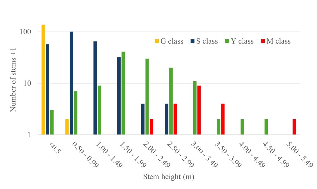
In 2023, 75% of stems had a single growth point, fewer than 5% had >10 growth points, and less than 1% had >20 growth points. The mean height of all S, Y, and M class stems in 2023 was 1.54 m (SE = 0.05 m), and the average number of growth points was 2.1 growth points/stem (SE = 0.13 growth points/stem). Stems were relatively short: 61% were ≤1.0 m, while 4.4% were ≥3.0 m and 0.6% were ≥4.0 m. The tallest unbranched S class stem was 2.8 m, the shortest Y class stem was 0.6 m, and the shortest M class stem was 1.8 m. The tallest stem we measured was 5.3 m. Stem height within classes was variable, and the heights of stems in different stage classes overlapped considerably (Fig. 7). For example, 3% of S class stems were ≥2 m, while 38% of Y class stems and 17% of M class stems were ≤ 2.0 m.

Growth and Branching Dynamics

During our study, approximately 68% of stems showed positive growth rates >1 cm/yr, 17% showed negative growth rates, and about 15% of stems showed growth rates of <1 cm/yr (Fig. S2). Since negative growth and changes in number of growth point rates are a result of damage to the stem, we report negative rates separately from positive rates (all non-negative growth and change in number of growth point rates). The fit of the mixed effects model was low (Table S2A) and there was no significant association of positive growth rate with any environmental variable that we evaluated (Table S2B). The average annual positive growth rate of all stems was 2.7 cm/yr (95% CI = 2.4–3.0 cm/yr). There was no significant relationship between positive growth rate and initial stem height (R² = 0.24, F_{1, 297} = 0.70, P = 0.403), and there was no significant difference in the average annual positive growth of stems in different stage classes (F_{2, 295} = 0.99, P = 0.396).

During our study, 17% of stems decreased in height; negative growth rates averaged –6.4 cm/yr (95% CI = –4.9– –7.9 cm/yr) (Fig. S2). The fit of the mixed effects model for negative growth rates was greater than that of the positive growth rate model (Table S2A) but there were no significant associations with environmental variables we tested (Table S2B). However, 75% of stems that decreased in height were located in canyon plots. Annual average negative growth rates varied significantly with initial stem height (R² = 0.11, F_{1, 57} = 7.38, P = 0.009), with taller stems exhibiting more negative rates. Average annual negative growth rates also varied significantly across stage classes (F_{2, 56} = 6.79, P = 0.002), with S, Y, and M class stems having average annual negative growth rates of -1.1 cm/yr, -5.9 cm/yr and -7.4 cm/yr, respectively.

The annual increase in the number of growth points averaged 0.06 growth points/yr (95% CI = 0.04–0.08 growth points/yr; Fig. S3). Over two-thirds of stems showed no change in the number of growth points, and only 15% exceeded an average increase of 0.1 growth point/yr. The fit of the mixed effects model was low (Table S3A), but mean annual precipitation (F_{1, 297} = 4.72, P = 0.031) and landscape position (F_{1, 297} = 3.60, P = 0.059) were associated with positive change in growth points rates (Table S3B). There was a significant positive relationship between the average annual increase in number of growth points and the initial height of the stem (R² = 0.27, F_{1, 306} = 113.88, P <0.001), with taller stems exhibiting a greater average increase in growth points each year. Stage classes had significantly different positive growth rates (F_{2, 304} = 34.68, P <0.001), with M class adding the most growth points each year on average and S class adding the least.

Eleven percent of the stems had a negative average annual change in growth points (Fig. S3). The average annual loss of growth points among these stems was –0.5 growth points/yr (95% CI = –0.4– –0.7 growth points/yr). The mixed effect model fit was greater for negative average annual change in growth points than for positive change in growth point rates (Table S3A). Mean annual temperature (F_{1, 39} = 3.94, P = 0.054) and landscape position (F_{1, 39} = 3.54, P = 0.068) were associated with negative changes in growth point rates (Table S3B). Eighty-two percent of stems that exhibited negative changes in growth point were in canyon plots. The average annual loss of growth points was significantly related to the initial height of the stem (R² = 0.15, F_{1, 48} = 8.67, P = 0.005), with taller stems exhibiting a more negative average annual loss rate. Explanatory variables included in the mixed-effects models were highly correlated with one another (Table S4), rather than with the response variable, and results should therefore be interpreted as associations rather than independent effects. Stage classes had significantly different negative average annual changes in growth point rates (F_{2, 47} = 26.54, P < 0.001), with M class having the most negative rates and S class the least negative rates. The environmental variables included in the mixed effects models were moderately to highly correlated, and all pairwise correlations were statistically significant (P < 0.001, Table S4).

Stage Class Transition and Regression Rates

Stage class structure changed substantially in some plots via production of G class stems, stem mortality, and transitions and regressions of stems to different stage classes. The number of stems transitioning from smaller to larger stage classes was low; on average, 2% of S class stems and 0.4% of Y class stems transitioned to the next larger stage class each year (Table 3). The average proportion of stems regressing to a smaller stage class was comparable to transition rates to larger classes; 1.7% of Y class stems regressed to S class and 5.6% of M class stems regressed to Y class each year. The average annual survival of S, Y, and M class stems was high (Table 3). Annual survival was particularly high for M class stems, with only two of 22 stems dying during the study period.

Table 3. Average annual demographic rates by stage class.

Stage Class	Annual Survival	Annual Mortality	Annual Transition	Annual Regression
S	0.979	0.021	0.019	NAa
Y	0.982	0.018	0.004	0.017
M	0.996	0.004	NAa	0.056

We did not tag G class stems until 2023 and thus cannot calculate class-specific survival and transition rates, but the numbers of G class individuals we observed over time illustrate the potential density dynamics of this stage class. The abundance of G class stems in specific plots both increased and decreased from 2018 to 2023, sometimes substantially (e.g., +15 stems and -25 stems, Table 2). Average density of G class stems trended higher over the course of our study but not significantly (t₁₄= 0.75, P = 0.464).

Discussion

 Population Structure

The clonal stands of Y. brevifolia in our study area are higher density and of lower stature than those described in other parts of its range (MacMahon 2000; Keeler-Wolf 2007). The average density of Y. brevifolia stems in our plots (2,170 stems/ha; Table 2) is an order of magnitude higher than densities of approximately 3 trees/ha to a high of 450 trees/ha reported from other portions of its range (Rowlands 1978; Vasek and Barbour 1978; St. Clair and Hoines 2018, Sweet et al. 2019; CDFW 2022). The variance of stem density in our plots is high (Table 2), suggesting the local distribution of Y. brevifolia is patchy at our sampling scale of 0.01 ha. Most stems in our study area are short, single-stemmed plants with a single growth point. The mean height (1.54 m) and maximum height (5.3 m) of our population are below reported Y. brevifolia mean heights (2.2–3.6 m; Vasek and Barbour 1978; Comanor and Clark 2000; Gilliland et al. 2006) and maximum heights (6–12.5 m; Rowlands 1978; Gilliland et al. 2006; CDFW 2022). The mean number of growth points in our study population (2.1 growth points/stem) is indicative of the dominance of stems with single growth points. While trees with many dozens of branches have been reported elsewhere (Simpson 1975; Gilliland et al. 2006), the maximum number of growth points in our study population is 28.

Size to first flowering is variable; the largest S class stem (i.e., stems that have not yet flowered) is 2.5 m and the smallest Y class stem (i.e., stems that have flowered at least once) is 0.7 m (Fig. 7). Twenty-nine S class stems flowered and transitioned to Y class during our study. The mean height of the S class stems prior to transition was 1.43 m and of those stems after transition was 1.63 m. If we assume that height at first-flowering occurred at the midpoint of that range, approximately 1.5 m, and we use the brackets of the 95% confidence interval around the average positive growth rate for our population (2.4 cm/yr, 3.0 cm/yr), then we estimate age at first-flowering was between 51 and 62 years in our study area. This is consistent with a generation time of 50–70 years estimated by other investigators (Esque et al. 2015). Similarly, the tallest stem in our population (5.3 m) would be between 177 and 221 years old, assuming constant growth and no regression of height. We observed no Y. brevifolia seedlings in our study plots. Given the apparent dominance of these stands by stems derived from rhizomes, the frequency that new genets are established from seed in this population is unknown, and fine-scale genetic information would help clarify the relative roles of sexual and asexual reproduction in this region. Our study area is approximately 40 km northwest of the type locality of forma herbertii, and our results are descriptive of Y. brevifolia exhibiting this low-growing, clumping, rhizomatous growth habit (Webber 1953), which also occurs along other parts of the western leading edge of Y. brevifolia’s range (Fig. 4).

Growth and Branching Dynamics

The average annual positive growth rate of Y. brevifolia stems in our plots (2.7 cm/yr) is comparable to mean growth rates of 3–4 cm/yr reported elsewhere (Comanor and Clark 2000; Gilliland et al. 2006; Esque et al. 2015), but growth rates in our study area are variable, with 35% of tagged stems growing at rates of ≤1 cm/yr. The average annual increase in growth points is low (0.06 growth point/yr), and no stem exceeded an average annual increase of 1.0 growth point/yr. This indicates flowering occurred infrequently during the short timeframe of our study, as typically Y. brevifolia produces two to three new growth points following the loss of an apical growth point to flowering (Simpson 1975). Most of the stems in our study population are S class that have never flowered and did not increase their number of growth points (Figure 7). We found no relationship between stem height, stage class, or landscape position and average annual growth rate or increase in growth points.

We suggest that wind is a significant disturbance process affecting Y. brevifolia size, architecture, and growth in this landscape. In our study many stems regressed in size (Figs. S2 and S3); 17% of stems had negative average annual growth rates and 10% of stems had negative average annual changes in their number of growth points. Taller stems with more growth points had higher average annual negative changes in both growth and change in growth point rates. Canyon plots appear to be associated with higher negative change in growth point rates than plots on alluvial fans, and stems with negative growth and change in growth point rates occur more frequently in canyon plots. The Tehachapi Mountains and the Transverse Ranges generate mountain wave front winds on their lee sides that flow down into the Antelope Valley (Zambrano 1980). Wind velocities >17 m/second (Beaufort Scale No. 8, gale force) can cause trees to sway and limbs to break, and velocities >25 m/second (Beaufort Scale No. 10, storm force) can uproot trees. In the Antelope Valley over the past 17 years, an average of >150 potentially damaging gale force wind gusts have been recorded each year, with an average of >60 gusts each year exceeding storm force. Leaf and branch shedding by trees can be adaptive in windswept landscapes as a way of reducing wind stress on the tree and the potential for uprooting (Mitchell 2013) but creates uncertainty around the true age of wind-damaged Y. brevifolia stems if height and number of growth points are used as proxies for age.

Stage Class Transition and Regression Rates

The production of G class stems is dynamic across both time and space, with almost all the G class stems appearing to be vegetative sprouts from rhizomes produced by parent stems. Some S class stems are far enough away from a potential parent plant that there is a high probability that they established from seed. However, given the abundance of young stems around fewer larger stems, rhizomatous stem production likely dominates in this landscape. Some plots exhibit large changes in G class stem number over a short period (e.g., 5 years), suggesting a potentially high production of rhizomes, as well as a potentially high mortality rate. G class stems that we excavated were connected to a parent plant by a rhizome. In one case, the rhizome had forked and new stems were growing from underground buds on the rhizome. We also observed scars where an old rhizome may have started to grow and died. Thus, a single rhizome can create a network of new G class stems, while others may be more ephemeral. Rhizomes can vary in their density, architecture, growth, and survival just as above-ground stems (Simpson 1975), creating additional uncertainty in our understanding of clonal Joshua tree population dynamics.

While taller stems have a higher survival rate in this landscape, damage from wind is continually breaking branches and pushing those stems back to a smaller stage class (Table 3). Survival of S class stems is lower than Y or M class stems, and on average only 2% of the S class stems flowered, branched, and transitioned to Y class each year of our study. Although rare in our population, survival is highest for M class stems, but their regression rate exceeds the Y class to M class transition rate (Table 3).

Frequent rhizome production, stem damage, and resprouting complicate assessing the true age structure of these stands, and their size structure and architecture are spatially and temporally dynamic. A larger M class stem may continually be broken or top-killed, then resprout and regrow following the damage, making the original “individual” or genet difficult to age from its architecture. Clonal stems surviving a mother stem grow, flower, branch, and serve as potential mother stems for future clones. The abundance of G class clones can quickly increase and, if those clones survive, the population can increase much more quickly than in populations that rely primarily on seedlings for recruitment because flowering is infrequent in Y. brevifolia and seedling survival is low (Esque et al. 2015). We did not conduct focused seedling surveys, which could help assess the level of recruitment from seedlings, but recruitment events are likely infrequent, requiring very long-term monitoring. Fine-scale genomic information on the population may help elucidate the level of recruitment derived from sexual reproduction, but past recruitment levels may not predict future levels given the changing climate. Better estimates of G class dynamics would help to quantify G class to S class transition rates and the potential for vegetative recruitment of larger stems into the population.

The stage class population model presented here (Fig. 3) could be used to describe stage dynamics and potential stand architecture in these Y. brevifolia populations once we have complete estimates of stage-specific transition and regression rates. However, to understand the true age-structured population dynamics, we must understand the dynamics of genets versus that of ramets and refine survival estimates of stems to account for resprouting. If a stem dying above ground is replaced by rhizomes produced by that stem, then actual survival of individuals is likely higher than we estimated, and a genet may live as long as its clones continue to produce rhizomes and additional clones.

Biogeography

Webber (1953) described dense, short stature rhizomatous stands in the western Antelope Valley as a distinct form of Y. brevifolia, “forma herbertii.” While not a valid taxon (Baldwin et al. 2012), this was one of the first descriptions of the rhizomatous growth form of Y. brevifolia, which Webber (1953) said ranged along the front of the Tehachapi Mountains to at least Monolith, California. The distribution of the rhizomatous growth form of Y. brevifolia has not been quantified. VegCAMP has mapped 76 km² of high (>5%) cover Y. brevifolia stands across a portion of its range in California (CDFW 2015, 2021, 2024), which overlap with some of the high density stands in our study area (Fig. 4). We believe these mapped high cover stands, which occur along the bajadas and alluvial fans of the southern Sierra Nevada, San Gabriel Mountains, and Tehachapi Mountains, are largely the rhizomatous “forma herbertii” described by Webber (1953) and documented in this study. Available vegetation maps do not extend to the upper elevations of the ranges of the high cover stands of Y. brevifolia, but the mapped stands appear to occur at its western range margins (Fig. 4). Webber (1953) reported this growth form to occur in high elevation areas of the species range. In mapped areas supporting high cover populations, winter rainfall is high, summer rainfall is low, and minimum and maximum temperatures are moderate (Fig. 6).

Resprouting and rhizome production of Y. brevifolia have been documented following damage from fires (Loik et al. 2000; DeFalco et al. 2010) and the rhizomatous growth form is generally considered to be a response to frequent fires (Keeler-Wolf 2007). Survival of post-fire resprouts is greater in higher elevation areas, however; and sprouting and rhizomatous stem production also occur independently of fire (e.g., DeFalco et al. 2010) as we have documented in this study. Fire return intervals vary substantially across the likely range of the rhizomatous growth form (USDA 2016). In higher elevation areas where Y. brevifolia grows in association with chaparral, scrub oak, and pine forest communities, fire return intervals are less than 100 years. Repeated fires preventing stems from reaching heights observed in other populations could explain the size distribution of stems in the region, and fires at significantly less than 50–60-year intervals could prevent stems from reaching maturity and explain the dominance of short stems. However, the rhizomatous growth form extends down into mid-elevation Mojave mixed desert scrub communities where fire return intervals exceed 400 years. If fire were a strong driver of structure in these stands, we would expect to find a mosaic of stand architecture, which we did not observe in our study area.

While many low-elevation desert Yucca species produce rhizomes (Webber 1953), cloning in some plant taxa appears to be more frequent in cold, wet, nutrient-poor, and low light environments (van Groenendael et al. 1996). Webber (1953) also hypothesized that rhizome production of Y. brevifolia was greater in wetter environments. Rhizome production stimulated by the wetter conditions present at the western edge of the species’ range may be a factor in the development of the rhizomatous growth form. In addition, we documented stem and branch damage occurring in approximately 1% of stems each year, presumably from high Tehachapi Mountain front winds. Webber (1953) speculated stem damage could stimulate rhizome production and might explain some of the dense patches of clonal stems he observed. We believe that damage from mountain-front winds at the western edges of Y. brevifolia’s range likely plays a role in shaping its population ecology and stand architecture. However, the relative roles of these factors in producing the rhizomatous growth form observed at the western edge of Y. brevifolia’s range is unclear and merits additional research.

Acknowledgments

The Tejon Ranch Company provided access to the conserved lands of its property for this research. We thank F. Davis for his helpful review of a draft manuscript. J. Stallcup and four anonymous reviewers made valuable technical and editorial suggestions that improved the final paper. J. Palmer made the maps and provided GIS support. We thank the 2010 Whitman College Semester in the West class for their assistance in initially establishing some of our study plots, and the various Conservancy staff, docents, and interns that have assisted with data collection over the years. The Tejon Ranch Conservancy provided funding for this research.

Literature Cited

• Baldwin, R. E., D. H. Goldman, and L. A. Vorobik, editors. 2012. The Jepson Manual: Vascular Plants of California. 2nd edition. University of California Press, Berkeley and Los Angeles, CA, USA.
• Barrows, C. W., and M. L. Murphy-Mariscal. 2012. Modeling impacts of climate change on Joshua trees at their southern boundary: how scale impacts predictions. Biological Conservation 152:29–36.
• California Department of Fish and Wildlife (CDFW). 2015. Proposed Tehachapi Pass high speed rail corridor vegetation map [ds1328]. Biogeographic Information and Observation System (BIOS). Available from: https://wildlife.ca.gov/Data/BIOS/Dataset-Index (Accessed: August 2022)
• California Department of Fish and Wildlife (CDFW). 2021. Vegetation: Owens Valley and Jawbone [ds2874]. Biogeographic Information and Observation System (BIOS). Available from: https://wildlife.ca.gov/Data/BIOS/Dataset-Index (Accessed 16 September 2024)
• California Department of Fish and Wildlife (CDFW). 2022. A status review of western Joshua tree (Yucca brevifolia). Report to the Fish and Game Commission, California Natural Resources Agency, Sacramento, CA, USA.
• California Department of Fish and Wildlife (CDFW). 2024. Vegetation: Mojave Desert for DRECP, Final [ds735]. Biogeographic Information and Observation System (BIOS). Available from: https://wildlife.ca.gov/Data/BIOS/Dataset-Index (Accessed 16 September 2024)
• California Department of Fish and Wildlife (CDFW). 2025. Western Joshua Tree Conservation Plan. Draft presented to the California Fish and Game Commission, California Natural Resources Agency, Sacramento, CA, USA.
• California Department of Forestry and Fire Protection (CAL FIRE). 2025. ). California Fire and Resource Assessment Program. Historical fire perimeters. https://www.fire.ca.gov/what-we-do/fire-resources-assessment program/fire-perimeters
• California Regional Water Quality Control Board (CRWQCB). 2021. Water quality control plan for the Lahontan region, CA. CRWQCB, Lahontan Region, South Lake Tahoe, CA, USA.
• Cleland, D. T., J. A. Freeouf, J. E. Keys, G. J. Nowacki, C. A. Carpenter, and W. H. McNab. 2007. Ecological Subregions: Sections and Subsections for the conterminous United States. General Technical Report WO-79D [Map on CD-ROM] (A. M. Sloan, cartographer). U.S. Department of Agriculture, Forest Service, Washington, D.C., USA.
• Cole, K. L., K. Ironside, J. Eischeid, G. Garfin, P. B. Duffy, and C. Toney. 2011. Past and ongoing shifts in Joshua tree distribution support future modeled range contraction. Ecological Applications 21(1):137–149.
• Comanor, P. L., and W. H. Clark. 2000. Preliminary growth rates and a proposed age-form classification for the Joshua tree, Yucca brevifolia (Agavaceae). Haseltonia 7:37–46.
• Conover, W. J., and R. L. Iman. 1981. Rank transformations as a bridge between parametric and nonparametric statistics. The American Statistician 35(3):124–129.
• Crowe, E. 1957. Men of El Tejon: Empire in the Tehachapis. The Ward Ritchie Press, Los Angeles, CA, USA.
• DeFalco, L. A., T. C. Esque, S. J. Scoles-Sciulla, and J. Rodgers. 2010. Desert wildfire and severe drought diminish survivorship of the long-lived Joshua tree (Yucca brevifolia; Agavaceae). American Journal of Botany 97(2):243–250.
• Dibblee, T.W. 1963. Geology of the Willow Springs and Rosamond Quadrangles, California. Geological Survey Bulletin 1089-C. United States Government Printing Office, Washington, D.C., USA.
• Dibblee, T. W. 2008. Geologic map of the Neenach and Willow Springs quadrangles. Dibblee Geology Center Map #DF-383. Santa Barbara Museum of Natural History, Santa Barbara, CA, USA.
• Esque, T. C., P. A. Medica, D. F. Shryock, L. A. DeFalco, R. H. Webb, and R. B. Hunter. 2015. Direct and indirect effects of environmental variability on growth and survivorship of pre-reproductive Joshua trees, Yucca brevifolia Engelm. (Agavaceae). American Journal of Botany 102(1):85–91.
• Esque, T. C., D. F. Shryock, G. A. Berry, F. C. Chen, L. A. DeFalco, S. M. Lewicki, B. L. Cunningham, E.J. Gaylord, C.S. Poage, G.E. Gantz, R.A. Van Gaalen, B.O. Gottsacker, C.J. Smith, and K.E. Nussear. 2023. Unprecedented distribution data for Joshua trees (Yucca brevifolia and Y. jaegeriana) reveal contemporary climate associations of a Mojave Desert icon. Frontiers in Ecology and Evolution 11:1266892. www.doi.org/10.3389/fevo.2023.1266892
• Gilliland, K. D., N. J. Huntly, and J. E. Anderson. 2006. Age and population structure of Joshua trees (Yucca brevifolia) in the northwestern Mojave Desert. Western North American Naturalist 66(2):art6.
• Gucker, C. L. 2006. Yucca brevifolia. In: Fire Effects Information System [Online]. Fire Sciences Laboratory, Rocky Mountain Research Station, U.S. Department of Agriculture, Forest Service. Available from: https://www.fs.usda.gov/database/feis/plants/tree/yucbre/all.html (Accessed: 31 October 2024)
• Keeler-Wolf, T. 2007. Mojave Desert scrub vegetation. Pages 609–656 in M. G. Barbour, T. Keeler-Wolf, and A. A. Schoenherr, editors. Terrestrial Vegetation of California. 3rd edition. University of California Press, Berkeley and Los Angeles, CA, USA.
• Latta, F. F. 1976. Saga of Rancho El Tejón. Bear State Books, Santa Cruz, CA, USA.
• Lenz, L.W. 2007. Reassessment of Yucca brevifolia and recognition of Y. jaegeriana as a distinct species. Aliso 24(1):97–104.
• Loik, M. E., C. D. St. Onge, and J. Rodgers. 2000. Post-fire recruitment of Yucca brevifolia and Yucca schidigera in Joshua Tree National Park, California. Pages 79–85 in J. E. Keeley, M. Baer-Keeley, and C. J. Fotheringham, editors. 2nd Interface Between Ecology and Land Development in California. U.S. Geological Survey Open-File Report 00-62. U.S. Geological Survey, Western Ecological Research Center, Sacramento, CA, USA. https://doi.org/10.3133/ofr0062
• MacMahon, J. A. 2000. Warm deserts. Pages 285–322 in M. G. Barbour, and W. D. Billings, editors. North American Terrestrial Vegetation. 2nd edition. Cambridge University Press, New York, NY, USA.
• McKelvey, S. D. 1938. Yuccas of the southwestern United States, I. Arnold Arboretum of Harvard University, Jamaica Plain, MA, USA.
• Mitchell, S. J. 2013. Wind as a natural disturbance agent in forests: a synthesis. Forestry 86:147–157. https://doi:10.1093/forestry/cps058
• PRISM Climate Group. 2021. Oregon State University. Available from: https://prism.oregonstate.edu (Accessed: September 2024)
• Reynolds, J. R., and D. K. Nagami. 2011. Lines in the sand: contrasting advocacy strategies for environmental protection in the twenty-first century. UC Irvine Law Review 1(4):1124–1166.
• Rowlands, P. G. 1978. The vegetation dynamics of the Joshua tree (Yucca brevifolia Engelm.) in the southwestern United States of America. Dissertation, University of California, Riverside, CA, USA.
• Royer, A. M., M. A Streisfeld, and C. I. Smith. 2016. Population genomics of divergence within an obligate pollination mutualism: selection maintains differences between Joshua tree species. American Journal of Botany 103(10):1730–1741.
• Sawyer, J. O., T. Keeler-Wolf, and J. M. Evans. 2009. A Manual of California Vegetation. 2nd edition. California Native Plant Society, Sacramento, CA, USA.
• Shryock, D. F., T. C. Esque, G. A. Berry, and L. A. DeFalco. 2025. Assessing uncertainty in forecasts of refugia for Jushua trees using high-density distribution data. Ecosphere 16(6):e70308. https://doi.org/10.1002/ecs2.70308
• Simpson, P. G. 1975. Anatomy and morphology of the Joshua tree (Yucca brevifolia): an arborescent monocot. Dissertation, University of California, Santa Barbara, CA, USA.
• St. Clair, S. B., and J. Hoines. 2018. Reproductive ecology and stand structure of Joshua tree forests across climate gradients of the Mojave Desert. PLOS ONE 13(2):e0193248. https://doi.org/10.1371/journal.pone.0193248
• State of California. 2023. Western Joshua Tree Conservation Act. A table bill to the California State Legislature. SECTION 1. Chapter 11.5 (commencing with section 1927) is added to Division 2 of Fish and Game Code.
• Sweet, L. C., T. Green, J. G. C. Heintz, N. Frakes, N. Graver, J. S. Rangitsch, J. E. Rodgers, S. Heacox, and C. W. Barrows. 2019. Congruence between future distribution models and empirical data for an iconic species at Joshua Tree National Park. Ecosphere 10(6):e02763. https://doi.org/10.1002/ecs2.2763
• U.S. Department of Agriculture (USDA). 2016. LANDFIRE 2016 Remap Fire Return Interval for the Continental United States. Available from: https://www.landfire.gov
• U.S. Fish and Wildlife Service (USFWS). 2023a. Endangered and Threatened Wildlife and Plants; Petition Finding for Joshua Trees (Yucca brevifolia and Y. jaegeriana). Federal Register 88(46):14536–14537.
• U.S. Fish and Wildlife Service (USFWS). 2023b. Species Status Assessment Report for the Joshua Tree (Yucca brevifolia). Version 2.0, February 2023. U.S. Fish and Wildlife Service, Pacific Southwest Region, Sacramento, CA, USA.
• Van Groenendael, J. M., L. Klimeš, J. Klimesova, and R. J. J. Hendriks. 1996. Plant life histories: ecological correlates and phylogenetic constraints. Philosophical Transactions of the Royal Society of London 351:1331–1339.
• Vasek, F. C., and M. G. Barbour. 1978. Mojave Desert scrub vegetation. Pages 835–868 in M. G. Barbour and J. Major, editors. Terrestrial Vegetation of California. Special Publication Number 9. University of California Press, Berkeley and Los Angeles, CA, USA.
• Webber, J. M. 1953. Yuccas of the Southwest. Agriculture Monograph No. 17, U.S. Department of Agriculture. Washington, D.C., USA.
• Western Regional Climate Center (WRCC). 2024. Maximum wind gust hourly observations 1995-2023. Available from: https://wrcc.dri.edu/cgi-bin/rawMAIN.pl?caCPOP (Accessed: 21 October 2024)
• White, M. D., E. R. Pandolfino, and A. Jones. 2011. Purple martin survey results at Tejon Ranch in the Tehachapi Mountains of California. Western Birds 42(3):164–173.
• White, M. D., and K. Penrod. 2012. The Tehachapi connection: a case study of linkage design, conservation, and restoration. Ecological Restoration 30(4):279–282.
• Wilkening, J. L., S. L. Hoffmann, and F. Sirchia. 2020. Examining the past, present, and future of an iconic Mojave Desert species, the Joshua tree (Yucca brevifolia, Yucca jaegeriana). Southwestern Naturalist 65:216–229.
• Zambrano, T. G. 1980. Assessing the Local Windfield with Instrumentation. Prepared for Pacific Northwest Laboratory Under Agreement B-92864-A-H. Pacific Northwest Laboratory, Operated for the U.S. Department of Energy by Battelle Memorial Institute. PNL-3622/UC-60.