Identifying highly used Dungeness crab fleet fishing areas off central and northern California to inform entanglement risks of large whales
FULL RESEARCH ARTICLE
Michael Johns1*, Kathi George2, Rebekah Lane2, and Jaime Jahncke1
1 Point Blue Conservation Science, 3820 Cypress Drive, Suite 11, Petaluma, CA 94954, USA https://orcid.org/0000-0002-0295-5121 (MJ) https://orcid.org/0000-0002-2896-6101 (JJ)
2 The Marine Mammal Center, 2000 Bunker Road, Sausalito, CA 94965, USA https://orcid.org/0009-0002-9139-9362 (KG) https://orcid.org/0000-0002-7377-4360 (RL)
*Corresponding Author: mjohns@pointblue.org
Published 22 May 2026 • doi.org/10.51492/cfwj.112.5
Abstract
Large whales seasonally aggregate into highly productive areas to feed, which often overlap with regions popular for various fishing activities. This spatial and temporal overlap can lead to whale entanglements in fishing gear. Along the California coast, such impacts have been amplified by intense marine heat waves and climate-driven shifts in whale migration and habitat use, resulting in unprecedented reports of entangled whales and substantial disruptions to the region’s valuable Dungeness crab fishery. In response, the Risk Assessment and Mitigation Program (RAMP) was established to reduce entanglement risk through collaboration and adaptive management. As part of this program, we sought to quantify the spatial footprint of crabbing effort in California waters. To achieve this, we analyzed solar logger positional data collected from a sample of commercial crabbing vessels in Central and Northern California, applying movement models adapted from animal behavior studies to identify where crabbing occurred. We then fitted resource selection functions using environmental and operational variables predicted to influence crab fishing behavior, producing a spatial surface of crabbing probability. This information on the timing and location of crabbing activity enhances our understanding of fishing effort distribution and enables managers to implement targeted strategies that, when combined with whale distribution data, may reduce entanglement risk while maintaining optimal crabbing opportunities.
Key words: fisheries management, GPS tracking, Hidden Markov Model, human use, mitigation, resource selection
| Citation: Johns, M. K. George, R. Lane, and J. Jahncke. 2026. Identifying highly used Dungeness crab fleet fishing areas off central and northern California to inform entanglement risks of large whales. California Fish and Wildlife Journal 112:e5. |
| Editor: Helen Killeen, Marine Region |
| Submitted: 17 September 2025; Accepted: 29 December 2026 |
| Copyright: ©2026, Johns et al. This is an open access article and is considered public domain. Users have the right to read, download, copy, distribute, print, search, or link to the full texts of articles in this journal, crawl them for indexing, pass them as data to software, or use them for any other lawful purpose, provided the authors and the California Department of Fish and Wildlife are acknowledged. |
| Funding: Partial funding of Point Blue’s staff time provided by the Firedoll Foundation and the Paul Angell Foundation. |
| Competing Interests: The authors have not declared any competing interests. |
Introduction
Large whales in the Eastern North Pacific were nearly hunted to extinction, but the ending of commercial whaling and legislation aimed at protecting populations has resulted in increasing trends for some species. Gray whales (Eschrichtius robustus) that make a predictable coastal migration from their southern breeding grounds in Baja California Mexico to their northern feeding grounds in the Bering, Beaufort, and Chukchi Seas have likely reached pre-whaling numbers of between 15,000 to 30,000 individuals (Stewart et al. 2023) before dropping to 12,900 individuals in 2025 (Eguchi et al. 2025), passing along the California coast between October and April each year. The Mexico and Central American distinct population segments of humpback whales (Megaptera novaeangliae) that feed off the coast of California, Oregon, and Washington have steadily increased from an estimated 3,000 in 2002 to 8,000 individuals in 2021 (Cheeseman et al. 2024), though both populations remain on the Endangered Species List (Bettridge et al. 2015). A smaller but growing population of endangered blue whales (Balaenoptera musculus) that breed off Central America and feed off the U.S. west coast have increased at an estimated rate of 3% per year, with a likely population size of 1,600 individuals (NMFS 2018) .
The coastal upwelling regions off California, specifically the Gulf of the Farallones and Monterey Bay, are important foraging hot spots for large baleen whales. Humpback and blue whales, among other species, make seasonal movements to California waters in the spring to feed on abundant schools of forage fish and aggregations of krill, with peak numbers occurring in the area from May through September. Recent climate-driven changes in the distribution of forage fish have resulted in a spatial shift towards the coast and over the continental shelf (Santora et al. 2020). Additionally, trends over the last three decades show that blue and humpback whales are arriving to their northern California feeding grounds up to 120 days earlier in response to ocean warming and associated changes in prey availability (Ingman et al. 2021).
Vessel strikes and entanglement with fishing gear are major sources of mortality for whales in California waters (Bettridge et al. 2015; Raverty et al. 2024). Both earlier arrival and habitat compression towards the coast in these areas is concerning for whale entanglement because it increases the spatial and temporal overlap between large whales and human recreational and commercial use of the oceans (Feist et al. 2021). The commercial harvesting of Dungeness crab (Cancer magister) has been ongoing since the 1840s and is considered one of the largest and most lucrative fisheries on the west coast of the United States (Hankin et al. 2005; Rasmuson 2013). In the last several decades, increased regulation on other valuable species such as Pacific salmon and groundfish has reallocated fishing effort towards Dungeness crab (Hankin et al. 2005). The California Dungeness crab fishery historically ran from mid-November to mid-July and is considered a “derby fishery,” with more than 70% of annual landings taking place in the first six weeks after opening (Hackett et al. 2003).
In 2014, a record-breaking marine heatwave resulted in pervasive harmful algal blooms (HABs) throughout the year that made crab unsafe for human consumption, delaying the 2015/2016 Dungeness crab season until March 2016 (Santora et al. 2020). This coincided with the arrival of humpback and blue whales to their feeding grounds, and the northward migration of gray whales along the California coast, resulting in an unprecedented increase in reports of entangled whales in California (Santora et al. 2020; Saez et al. 2021). In recent years, whale entanglements off the California coast have ranged from 48 confirmed reports in 2016 to 13 confirmed reports in 2020 (NOAA 2017, 2025). In 2019 and 2020, the California Department of Fish and Wildlife (CDFW) closed the fishery early to help alleviate the risk of large whale entanglement (Ingman et al. 2021). An assessment of the economic impact of the closure in 2019 in the waters west of San Francisco and Monterey estimated that the Dungeness crab fishery revenue would have been $9.4 million higher than the ~ $30 million that was reported without the closures (Seary et al. 2022).
In response to this increase in whale entanglements, CDFW, in partnership with the California Ocean Protection Council and the National Marine Fisheries Service, established the California Dungeness Crab Fishing Gear Working Group (hereafter referred to as simply Working Group). This 20-member Working Group brought together a unique coalition of commercial and recreational fishers, environmental representatives, entanglement response network members, state and federal agencies, and scientists. The group helped develop a Risk Assessment and Mitigation Program (RAMP) pilot to identify levels of whale entanglement risk and determine the needs for pre-season and in-season management options to reduce the risk of entanglement. This framework was eventually adopted by CDFW to inform management (CDFW 2020a,b). A major objective of the Working Group was to determine the spatial patterns of crabbing effort in Californian waters by outfitting a subsample of the crabbing fleet with solar powered passive GPS data loggers. Passive data loggers collected real-time location information of vessels during the crabbing season at a regular fine-scale interval.
GPS data has been used to reveal fishing effort in Madagascan reef fishery (Behivoke et al. 2021), pelagic trawlers in the Bay of Biscay (Vermard et al. 2010), Indonesian long liners (Utama et al. 2021), and trawl fishery in Queensland, Australia (Peel and Good 2011), to name a few studies. Dungeness crab fishers were required to begin using electronic monitoring systems by the 2023–2024 crabbing season, and a volunteer solar logger program informed that requirement. Here, we use raw GPS data from the Dungeness crab fishing fleet equipped with GPS loggers to identify crabbing activity through movement models traditionally employed to identify behavioral states of animals. Locations identified as crabbing behavior from the movement tracks of vessels were then pooled to model areas where crabbing activity is most likely based on bathymetry, sea floor substrate, and proximity to the port of call. Our goal for this analysis was not to produce a definitive map of crabbing locations in California waters, but rather to present a pilot approach to modeling human crab fishing behavior, with the potential to apply our method to a larger sample of the crabbing fleet.
Methods
Data Collection
Solar-powered passive GPS loggers manufactured by Pelagic Data Systems (29mm x 188mm x 81mm, 350 g) were outfitted to volunteer commercial crabbing vessels to log GPS positions from individual fishing trips, defined as a complete round trip from a port or harbor. We determined crabbing effort (versus fishing for other targets) by either comparing the dates from GPS tracks to landing receipts or direct confirmation by the fishers. We used data from 14 vessels, spanning commercial fishing zones 1–4 in California between the Oregon border and Lopez Point to the south (Fig. 1). For context, the California commercial Dungeness crab fishery is estimated to include approximately 471 active participating vessels, of which 385–470 typically make landings in each season. Based on historical CDFW permit data, the broader fleet’s vessel size distribution (as represented by our sample fleet) is dominated by vessels between 9–15 m (30–50 ft) (~70%). Participating vessels in our study were homeported at 11 locations (Fig. 1), covering many of the major California Dungeness crab landing centers such as Crescent City, Eureka, Fort Bragg, Bodega Bay, San Francisco, Half Moon Bay, and Moss Landing. Notably, we did not have good coverage of ports in the Point Arena location. Because our sample consisted of ~3% of the estimated active fleet, comprising specific vessel sizes and ports, we interpret our results as reflective of participating fishers’ behavior, with explicit acknowledgement of potential bias in fleetwide inference. The loggers recorded data for the months of November through June from 2019 to 2021, resulting in a total of 468 trips. Note that a brief depth restriction of within 70 m was initiated for Zone 4 in 2021 from 16 to 26 December. Raw GPS locations from onboard loggers contained irregular sampling intervals at high temporal resolution (between 5 to 10 seconds on average), so we subsampled GPS positions to a uniform 5-minute interval using the package amt (Signer et al. 2019).
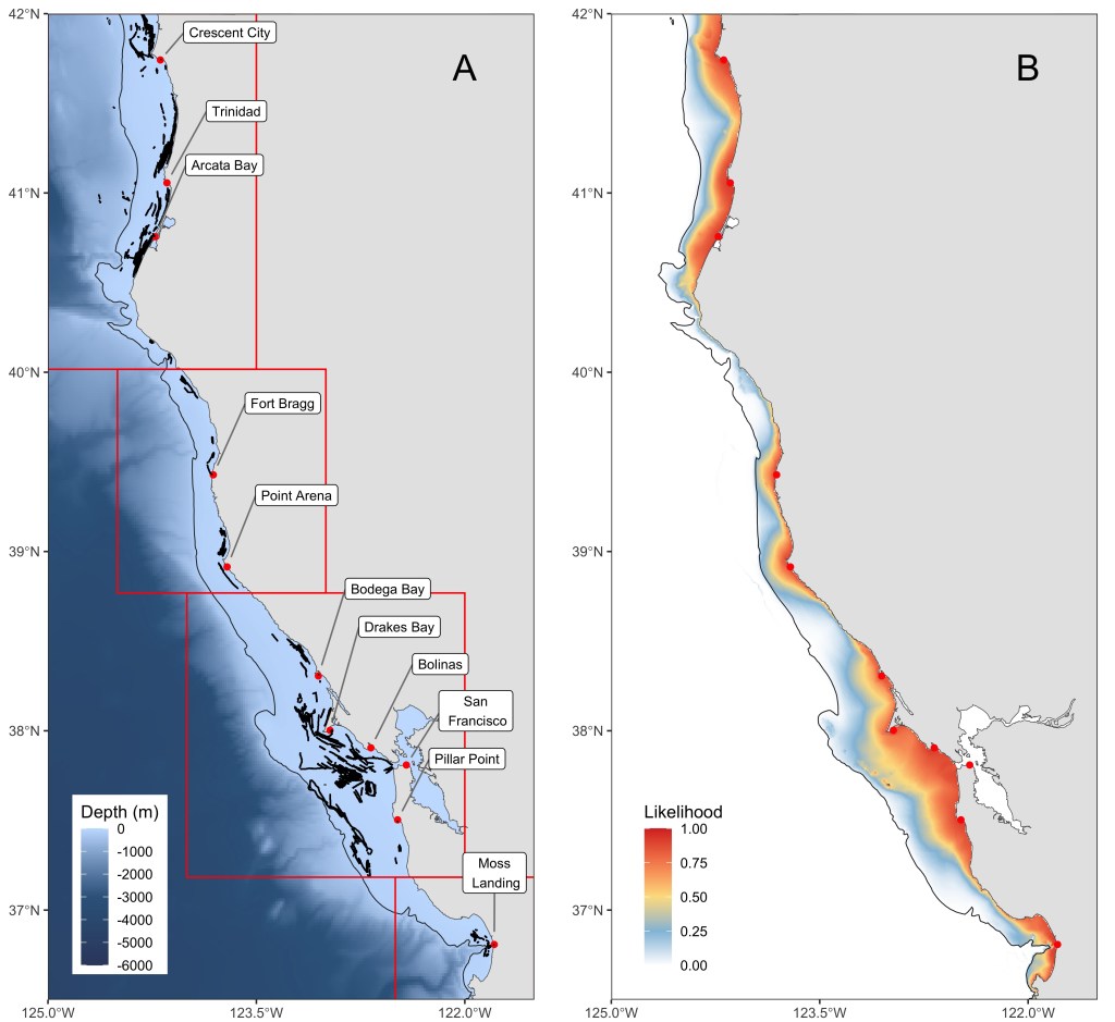
Figure 1. A) Overall map showing the locations of estimated crabbing behavior (black dots) from the 4-state HMM. Locations of ports or anchorages used by the 14 different vessels for crabbing trips are labeled. The four management zones are outlined in red. Depth is displayed in meters, with the 200-m continental shelf break as a thin solid line. B) Map depicting the likelihood surface of crabbing behavior using the coefficients of the top GLM model, with December as the reference month.
Identifying Crabbing Locations
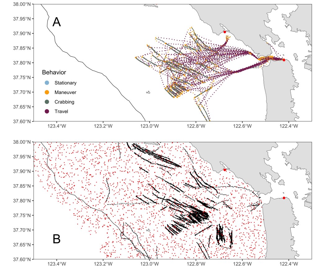
We calculated step lengths (sl), defined as the distance between each GPS position from time t to t+1 and turning angles (ta), defined as the bearing from the position at time t to the position at t+1, from the movement track of each trip. We specified a hidden Markov model (HMM) a priori based on our expectations of crabbing movements, with initial parameters for traveling (sl = 1000 meters, ta = 0.1 radian), maneuvering (sl = 20, ta = pi), and crabbing (sl = 500, ta = 0.2). These three states were generated with the assumption that vessels moved at longer steps while traveling and crabbing with turning angles concentrated near 0 while underway and deviating slightly from 0 when setting and pulling crab pots along a line. We assumed turning angles to be more tortuous when maneuvering, oscillating between –π and π, with smaller steps compared to traveling and crabbing. We fit a second HMM with an additional fourth state for stationary behavior at sea and near the port, with initial parameters (sl = 5, ta = pi). Akaike Information Criterion (AIC) from fitted HMMs were used to select the most parsimonious model. Vessel movement exhibits strong temporal dependence due to mechanical inertia, particularly at fine (5-min) sampling intervals. We fit the HMMs with the package moveHMM (Michelot et al. 2016) and evaluated model adequacy using multiple diagnostic approaches rather than model selection across different numbers of states. We assessed goodness of fit by examining pseudo-residuals for state-dependent distributions, checking for remaining autocorrelation and deviations from expected distributions. We evaluated state separation by examining overlap among state-dependent parameter estimates and assessed parameter stability by refitting the model using multiple sets of initial values. Each GPS position was assigned to one of the states from the final HMM (Fig. 2). The data were then filtered to only include points identified as actively crabbing.
Predicting Likelihood of Crabbing
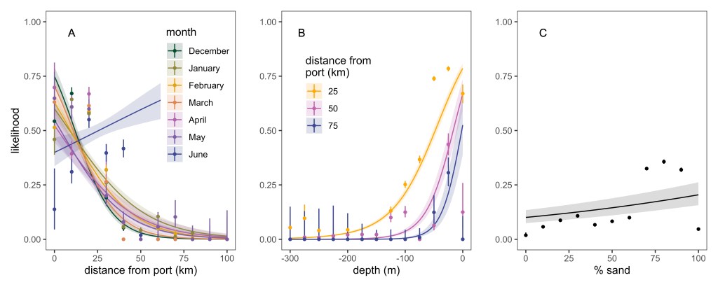
We predicted that Dungeness crab fishers relied on bathymetric information from onboard depth sounders and GPS units, and knowledge of bottom habitat type through experience and charts, when deciding where to place their crab pots. We predicted they would also account for monetary constraints such as the cost of fuel and the time it takes to transit the ocean given a reasonable speed of 8–10 knots, which would limit dispersal from their home ports to preferred crabbing locations. Finally, we assumed there would be a temporal element acting on distance traveled to selected crabbing locations, based on anecdotes that crabbing areas closer to ports become depleted as the season progresses, forcing crabbers to search for more far-reaching locations towards the end of the commercial crabbing season. Conversely, in some years based on crab abundance informed by recreational fishing effort, crabbing may occur in deeper water in early season and move closer to shore as the season progresses. Thus, to model the drivers of crabbing activity, we used the explanatory variables distance from port (meters from known ports and anchorages), a categorical month term, depth (in m), and the composition of seafloor substrate (% sand; Fig. 3). We retrieved raster layers depth and % sand through a public repository from a NOAA-funded analysis of deep-sea corals and sponges (Poti et al. 2023), with a 200 x 200 m spatial resolution that covered the entire California marine shelf down to 1,200 m depth. There were no significant correlations among continuous predictors described by Pearson correlation coefficients for depth:d2port r = –0.05, depth:%sand r = 0.5, and d2port:%sand r = – 0.05.

We assumed crabbing locations to be spatially structured along the California coast. We explicitly evaluated spatial autocorrelation in GLM residuals using Moran’s I and found strong dependence at short spatial lags. Rather than fitting fully spatial regression models, which can obscure inference on environmental covariates in this sort of study, we accounted for spatial structure using discrete coast-block effects and cluster-robust standard errors. All models included a factor term for discrete coast-block representing contiguous latitudinal fishing regions (20 uniform bins). This approach absorbs broad-scale spatial dependence and yields consistent coefficient estimates even in the presence of within-block correlation. We minimized temporal autocorrelation by aggregating locations at the monthly scale and by the used–available sampling design; remaining dependence is reflected in robust uncertainty estimates. Our inference therefore concerns covariate effects conditional on persistent fishing regions, rather than fine-scale spatial prediction.
For the response layer, we created a base spatial raster bounded by longitudes 125° and 121° W and latitudes 36° and 42.5° N with the same extent and resolution as the covariate layers, and coded pixels where crabbing was identified from the HMM process as “1.” A random sample (without replacement and excluding locations where crabbing occurred) equal to the number of pixels where crabbing did occur was drawn from the base spatial raster and coded as “0” for each month, representing locations where crabbing could have occurred but did not (pseudo unused locations; Fig. 2). We extracted explanatory variables for used (1) and unused (0) locations.
We fitted a candidate set of 30 generalized linear models (binomial family with logit link) with different combinations of the explanatory variables to predict the probability of crabbing behavior and ranked them by their resulting delta AICc corrected for small sample size (Burnham and Anderson 2002). The candidate set was defined a priori based on our hypotheses for the drivers of crabbing behavior rather than automated stepwise selection. We included an interaction between depth and distance to port to test for a possible tradeoff between these two parameters (vessels expected to crab closer to shore in areas where the shelf break was narrow for example), and a quadratic term for depth was included with the prediction that depths close to 0 or near the shelf break would not be preferred. Finally, we used an interaction between distance to port and month (factor) to address the prediction of differential preferences of dispersal limits throughout the crabbing season. Although models were ranked using AICc, we based final model interpretation on consistency of effect estimates, diagnostic performance, and robustness to spatial dependence rather than AIC alone. Cluster-robust standard errors with coast block as the clustering unit were used, allowing for consistent estimation of covariate effects while relaxing the assumption of independent observations within spatial blocks. We evaluated model fit using simulation-based residual diagnostics, including tests for deviations from the expected residual distribution, overdispersion, and spatial autocorrelation. To visualize where crabbing is likely to occur, we multiplied raster layers of retained explanatory variables with the coefficients of the top model and exponentiated the products to produce a likelihood surface of crabbing activity bounded by 0 (unlikely) and 1 (very likely).
Results
The 4-state Hidden Markov Model (HMM) received substantially stronger support than the 3-state model (ΔAIC = 20,876). The selected model identified four behavioral states based on step length and turning angle distributions (Fig. S1; Table S1). State 1 was characterized by short, right-skewed step lengths and highly variable turning angles (−π to π) and was classified as stationary. State 2 exhibited intermediate step lengths (centered ~520 m) with turning angles concentrated variable turning angles (−π to π) and was classified as maneuvering. State 3 showed shorter step lengths (centered ~370 m) with turning angles near 0 and was classified as crabbing. State 4 had longer step lengths (centered ~900 m) and turning angles concentrated near 0, consistent with directed traveling behavior. Pseudo-residuals were approximately normally distributed with no systematic deviations, indicating adequate fit of the state-dependent distributions (Fig. S2).
The model for predicting crabbing locations containing an interaction between distance to port and quadratic depth, an interaction between distance to port and month, and % sand received overwhelming support (cumulative AIC weight = 1; Table 1). The full model set is presented in Table S2. Simulation-based residual diagnostics indicated no strong deviations from the expected residual distribution (Kolmogorov–Smirnov test, P = 0.17), but detected residual overdispersion, consistent with spatial clustering of crabbing activity and the used–available study design. Diagnostic plots (residual–fitted and QQ plots) are provided in Figure S3. To ensure robust inference, we accounted for spatial dependence using coast-block effects and evaluated coefficient stability using cluster-robust standard errors (Table 2). The final model represents a spatially structured resource selection model describing where crabbing is likely to occur, conditional on persistent fishing regions and the small sample of volunteer vessels used to collect the use data.
Table 1. The top 10 models for predicting the likelihood of crabbing (crab ~) of the candidate set of 30 models, ranked from lowest ∆AICc to highest, with different relevant combinations of explanatory variables distance from port (d2port), depth, % sand (sand), and month. Number of parameters (K), AICc weight (wt), and log likelihood (LL) also reported.
| Model Formula | K | ΔAICc | Wt | LL |
| coast_block + depth*d2port + I(depth^2)*d2port + month*d2port + sand | 40 | 0.00 | 1 | –14695.44 |
| coast_block + depth*d2port + I(depth^2)*d2port + month*d2port | 39 | 110.99 | 0 | –14751.94 |
| coast_block + depth + I(depth^2) + month*d2port + sand | 38 | 147.74 | 0 | –14771.31 |
| coast_block + depth + I(depth^2) + month*d2port | 37 | 205.57 | 0 | –14801.23 |
| coast_block + depth + month*d2port + sand | 37 | 286.28 | 0 | –14841.58 |
| coast_block + depth*d2port + I(depth^2)*d2port + sand + month | 33 | 335.80 | 0 | –14870.35 |
| coast_block + depth + month*d2port | 36 | 369.97 | 0 | –14884.43 |
| coast_block + depth + I(depth^2) + sand + month | 31 | 408.62 | 0 | –14908.76 |
| coast_block + depth*d2port + I(depth^2)*d2port + month | 32 | 451.07 | 0 | –14928.99 |
| coast_block + depth + I(depth^2) + d2port + month | 30 | 483.82 | 0 | –14947.36 |
Table 2. Binomial GLM for predicting crabbing likelihood with cluster-robust standard errors (coast blocks), crab ~ coast_block + depth*d2port + I(depth2)d2port + monthd2port + sand. Coefficients are log-odds estimates from a binomial generalized linear model. Standard errors and P-values are based on cluster-robust covariance estimates with coast block as the clustering unit to account for spatial dependence among observations.
| Predictor | Estimate | Robust SE | Z-value | P-value |
| depth | 0.0135 | 0.00470 | 2.87 | 0.004 ** |
| distance to port (d2port) | 8.13 × 10⁻⁶ | 2.08 × 10⁻⁵ | 0.39 | 0.696 |
| depth² | 1.04 × 10⁻⁵ | 6.50 × 10⁻⁶ | 1.59 | 0.111 |
| December | 0.999 | 0.553 | 1.81 | 0.071 • |
| February | 0.429 | 0.497 | 0.86 | 0.387 |
| January | 0.311 | 0.482 | 0.65 | 0.518 |
| June | −0.504 | 0.624 | −0.81 | 0.419 |
| March | 0.767 | 0.529 | 1.45 | 0.147 |
| May | 0.102 | 0.645 | 0.16 | 0.875 |
| November | 1.96 | 1.81 | 1.08 | 0.280 |
| sand | 0.00833 | 0.00255 | 3.27 | 0.001 ** |
| depth × d2port | 5.88 × 10⁻⁷ | 1.67 × 10⁻⁷ | 3.51 | <0.001 *** |
| depth² × d2port | 4.15 × 10⁻¹⁰ | 1.79 × 10⁻¹⁰ | 2.32 | 0.020 * |
| d2port × December | −4.49 × 10⁻⁵ | 2.42 × 10⁻⁵ | −1.85 | 0.064 • |
| d2port × February | −9.99 × 10⁻⁶ | 2.08 × 10⁻⁵ | −0.48 | 0.631 |
| d2port × January | 3.42 × 10⁻⁷ | 2.01 × 10⁻⁵ | 0.02 | 0.986 |
| d2port × June | 6.24 × 10⁻⁵ | 2.46 × 10⁻⁵ | 2.54 | 0.011 * |
| d2port × March | −3.21 × 10⁻⁵ | 2.29 × 10⁻⁵ | −1.40 | 0.161 |
| d2port × May | −7.92 × 10⁻⁶ | 2.69 × 10⁻⁵ | −0.30 | 0.768 |
| d2port × November | −9.21 × 10⁻⁵ | 9.18 × 10⁻⁵ | −1.00 | 0.316 |
Across trips, vessels most frequently set pots in waters between 40 and 120 m depth. Crabbing locations occurred at distances of 16–20 km from the home port or anchorage on average, with modest seasonal variation in distance from port. Overall, the likelihood of crabbing declined with increasing distance from port, approaching zero beyond ~100 km. Crabbing was largely constrained within approximately 40 km of port or anchorage. Depth selection was non-linear, where vessels preferentially set gear at intermediate depths shallower than ~100 m, but these preferred depths were less likely to be used farther from port (Fig. 4). The addition of the interaction between distance to port and month was mainly driven by a significant positive effect on the likelihood of crabbing further from port in June, compared to a lower likelihood of crabbing with increasing distance from port for all other months (Table 2, Fig. 4). The habitat type sand was retained in the top model, with a slight increase in the likelihood of crabbing as the composition of % sand increased. We used predictions from the top model to generate a spatial likelihood surface for December as an example month (Fig. 1). These predictions reflect broad-scale patterns inferred from participating vessels and environmental covariates; however, localized or episodic offshore activity may occur in areas assigned low predicted probability.
Discussion
Changing ocean conditions have the potential to alter the distribution and abundance of both whales and fishing effort in unpredictable ways. We demonstrate that raw GPS tracks from a sample of vessels can provide a high-resolution and transparent method for determining where crabbing has and is most likely to occur. Applying well-tested movement models in this way can help managers identify high risk regions for whale entanglement and use this information to decrease the entanglement rate of whales while allowing the crab industry to provide for the market demand and retain a livelihood with reduced potential for endangering non-target species.
Our analysis highlights several key characteristics of crabbing activity in our study area, including non-linear relationships with depth and distance from port. Crabbing probability was largely constrained within ~40 km of port and declined sharply at greater distances. These spatial patterns are broadly consistent with previous reconstructions of Dungeness crab fishing effort along the U.S. West Coast derived from landing receipts, AIS data, and VMS data. In California, block-level effort surfaces developed from port landings data by Feist et al. (2021) and Free et al. (2023) similarly identified persistent nearshore concentrations of fishing effort within tens of kilometers of major ports. Qualitatively, our results align with these studies in showing a dominant nearshore footprint. Quantitatively, the steep decline in predicted crabbing probability beyond ~40 km from port in our analysis suggests a sharper spatial gradient than is apparent in block-aggregated effort estimates, likely reflecting differences in spatial resolution and modeling framework.
Seasonal redistribution patterns observed here are also comparable to those documented elsewhere on the West Coast. In Oregon and Washington, Riekkola et al. (2024) and Derville et al. (2023) reported shifts in effort distribution across months associated with environmental and management conditions. Our finding that vessels tend to set gear farther from port later in the season, particularly in June, is consistent with documented behavioral flexibility and spatial reorganization of the fleet under changing conditions (Liu et al. 2023).
One contrast emerges with respect to seafloor characteristics. While our model indicates a slight positive association with sandy substrates, Riekkola et al. (2024) reported greater fishing intensity in areas of higher rugosity in parts of the Pacific Northwest. These differences may reflect regional variation in substrate availability, bathymetry, and fleet behavior, but may also arise from differences in spatial resolution and modeling framework between gear-level GPS data and coarser effort reconstructions. The observed difference between Riekkola et al. (2024) and our work could also be an artifact of our relatively small sample size of vessels.
Differences between our results and prior effort reconstructions likely stem from both data source and modeling approach. Landing receipts provide long time series and fleet-wide coverage at the port level but lack spatial resolution. Technology like AIS and VMS record continuous vessel trajectories and enable broad-scale mapping, yet fishing activity must be inferred from movement characteristics and coverage may be incomplete for smaller vessels or when transponders are inactive. In contrast, solar loggers record high-resolution GPS tracks from participating vessels, and our estimates represent conditional probabilities of gear-setting at fine spatial scales rather than aggregated effort intensity. The finer resolution of solar logger data reveals heterogeneity within management blocks and sharper gradients in environmental and distance effects. These approaches are therefore complementary, where block-level and AIS/VMS-based analyses are well suited for fleet-wide and long-term assessment, whereas solar loggers provide detailed insight into vessel behavior and pot-level spatial patterns relevant to entanglement risk.
Participation in the solar logger project was limited during the study period, which overlapped with litigation affecting the California Dungeness crab fishery and likely reduced fleet participation and the representation of participating vessels and ports, as well as overlapping with the COVID-19 pandemic. Fourteen vessels across the study area participated, with some variation in percentage of each port and tier represented, whereas a maximum of 537 are permitted to fish in this area. This analysis illustrates the level of detail possible when using solar logger data to assess fishing activity; however, an increased sample of vessel movement data is needed to develop improved predictions of crabbing activity and monitor risk levels to marine life. Real-time GPS and cellular connectivity enabled fisheries monitoring units, such as Archipelago EM units, have been approved for use in the California Dungeness fleet beginning in 2023, and full implementation of the requirement began in November of 2025, which will provide the necessary data for improved monitoring at a temporal resolution of one minute. Increased fisher participation is vital in improving our understanding of fine-scale fishing activity and can be coupled with other data sources such as AIS, VMS, and landing receipts to better understand fishing intensity and broad-scale spatial distribution. Rather than replace existing approaches, solar loggers provide a complementary data source that can resolve individual vessel behaviors at high temporal resolution.
Modifications could be made to this analysis to refine patterns in the variance explained by time of year, annual trends, and location to ports and anchorages. Including a random term for vessel ID could account for differences in crabbing preferences explained by individual people or boats (favorite spots, differences in vessel performance or range, for example) and should be explored if this work is expanded in the future. In addition to producing a likelihood surface of crabbing use, it would be informative to include predictions of crabbing “intensity”, or the expected density of pots for a given location at a given time of year. To verify model predictions and confirm the accuracy of assigned behavioral states, future efforts should be made to ground truth these parameters by consulting with crab fishers directly, to survey where individuals set their pots and compare against the likelihood surfaces and behavior classifications generated with this modeling framework.
Results from this work are useful in three primary ways. First, they demonstrate that movement modeling frameworks commonly used to characterize animal behavioral states and habitat preferences, such as Hidden Markov Models and resource selection functions, can be applied to vessel GPS data to reveal specific fishing behaviors and predict preferred crabbing habitat. Second, model coefficients can be used to produce spatially explicit “hot spot” maps for vessels departing different ports under varying seasonal and environmental conditions. Finally, a dynamic workflow that ingests new GPS data could generate updated crabbing prediction maps to inform entanglement risk mitigation along the California coast. With continued engagement from agencies and commercial fishers, this framework can be refined to improve predictions of how crabbing behavior shifts across months, seasons, and regions.
Acknowledgments
We are especially grateful to the anonymous fishers who voluntarily and openly shared their fishing effort and vessel activity with our team. We thank Lindsay Caldwell and Ryan Bartling for comments on the manuscript. We also thank the California Ocean Protection Council (OPC) for funding the solar logger pilot project, the commercial Dungeness crabbers who participated in the project, especially Dick Ogg, and the Working Group for their support during the pilot phase. We also thank the Firedoll Foundation and the Paul Angell Foundation for their generous support, which partially funded Point Blue’s staff time on this project. This is Point Blue Contribution #2561. No large language models were used to generate any of the text or code in this manuscript.
Literature Cited
- Behivoke, F., M.-P. Etienne, J. Guitton, R. M. Randriatsara, E. Ranaivoson, and M. Léopold. 2021. Estimating fishing effort in small-scale fisheries using GPS tracking data and random forests. Ecological indicators 123:107321.
- Bettridge, S. O. M., C. S. Baker, J. Barlow, P. Clapham, M. J. Ford, D. Gouveia, D. K. Mattila, R. M. Pace, P. E. Rosel, and G. K. Silber. 2015. Status review of the humpback whale (Megaptera novaeangliae) under the Endangered Species Act. National Oceanic and Atmospheric Administration, National Marine Fisheries Service, Southwest Fisheries Science Center, La Jolla, CA, USA.
- Burnham, K. P., and D. R. Anderson. 2002. Model Selection and Multimodel Inference: A Practical Information-Theoretic Approach. 2nd edition. Springer, New York, NY, USA.
- California Department of Fish and Wildlife (CDFW). 2020a. Standardized Regulatory Impact Assessment. Proposed Addition of Section 132.8, Title 14, California Code of Regulations for the Risk Assessment Mitigation Program: Commercial Dungeness Crab Fishery. CDFW, Sacramento, CA, USA. https://dof.ca.gov/media/docs/forecasting/economics/major-regulations/major-regulations-table/CDFW_SRIA_Dungeness_Crab_Fishery.pdf
- California Department of Fish and Wildlife (CDFW). 2020b. Section 132.8. Risk Assessment Mitigation Program: Commercial Dungeness Crab Fishery. CDFW, Sacramento, CA, USA. https://nrm.dfg.ca.gov/FileHandler.ashx?DocumentID=184189&inline
- Cheeseman, T., J. Barlow, J. M. Acebes, K. Audley, L. Bejder, C. Birdsall, O. S. Bracamontes, A. L. Bradford, J. Byington, and J. Calambokidis. 2024. Bellwethers of change: population modelling of North Pacific humpback whales from 2002 through 2021 reveals shift from recovery to climate response. Royal Society Open Science 11:231462.
- Derville, S., T. V Buell, K. C. Corbett, C. Hayslip, and L. G. Torres. 2023. Exposure of whales to entanglement risk in Dungeness crab fishing gear in Oregon, USA, reveals distinctive spatio-temporal and climatic patterns. Biological Conservation 281:109989.
- Eguchi, T., A. Lang, and D. Weller. 2025. Abundance of eastern North Pacific gray whales 2024/2025. NOAA Technical Memorandum NMFS-SWFSC-724. National Oceanic and Atmospheric Administration, National Marine Fisheries Service, Southwest Fisheries Science Center, La Jolla, CA, USA. https://doi.org/10.25923/jqea-s505
- Feist, B. E., J. F. Samhouri, K. A. Forney, and L. E. Saez. 2021. Footprints of fixed‐gear fisheries in relation to rising whale entanglements on the U.S. West Coast. Fisheries Management and Ecology 28:283–294.
- Hackett, S. C., M. J. Krachey, C. M. Dewees, D. G. Hankin, and K. Sortais. 2003. An economic overview of Dungeness crab (Cancer magister) processing in California. California Cooperative Oceanic Fisheries Investigations Report 86–93.
- Hankin, D. G., S. C. Hackett, and C. M. Dewees. 2005. California’s Dungeness Crab: Conserving the Resource and Increasing the Net Economic Value of the Fishery. Sea Grant Final Report. University of California, San Diego, CA, USA.
- Ingman, K., E. Hines, P. L. F. Mazzini, R. C. Rockwood, N. Nur, and J. Jahncke. 2021. Modeling changes in baleen whale seasonal abundance, timing of migration, and environmental variables to explain the sudden rise in entanglements in California. PLOS ONE 16:e0248557.
- Liu, O. R., E. J. Ward, S. C. Anderson, K. S. Andrews, L. A. K. Barnett, S. Brodie, G. Carroll, J. Fiechter, M. A. Haltuch, C. J. Harvey, E. L. Hazen, P. Hernvann, M. Jacox, I. C. Kaplan, S. Matson, K. Norman, M. P. Buil, R. L. Selden, A. Shelton, and J. F. Samhouri. 2023. Species redistribution creates unequal outcomes for multispecies fisheries under projected climate change. Science Advances 9(33):5468.
- Michelot, T., L. Langrock, and T. A. Patterson. 2016. moveHMM: an R package for the statistical modelling of animal movement data using hidden Markov models. Methods in Ecology and Evolution 7:1308–1315.
- National Marine Fisheries Service (NMFS). 2018. Draft Recovery Plan for the Blue Whale (Balaenoptera musculus) – Revision. National Oceanic and Atmospheric Administration, Silver Spring, MD, USA.
- National Oceanic and Atmospheric Administration (NOAA). 2025. West Coast Large Whale Entanglement Response Program. Available from: https://www.fisheries.noaa.gov/west-coast/marine-mammal-protection/west-coast-large-whale-entanglement-response-program
- Peel, D., and N. M. Good. 2011. A hidden Markov model approach for determining vessel activity from vessel monitoring system data. Canadian Journal of Fisheries and Aquatic Sciences 68:1252–1264.
- Poti, M., S. K. Henkel, J. J. Bizzarro, T. F. Hourigan, M. E. Clarke, C. E. Whitmire, A. Powell, M. M. Yoklavich, L. Bauer, A. J. Winship, M. Coyne, D. J. Gillett, L. Gilbane, J. Christensen, and C. F. G. Jeffrey. 2023. NCCOS Assessment: U.S. West Coast Cross-Shelf Habitat Suitability Modeling of Deep-sea Corals and Sponges, 2016-10-01 to 2020-09-30 (NCEI Accession 0276883). National Oceanic and Atmospheric Administration, National Centers for Environmental Information, Asheville, NC, USA.
- Rasmuson, L. K. 2013. The biology, ecology and fishery of the Dungeness crab, Cancer magister. Advances in Marine Biology 65:95–148.
- Riekkola, L., O. R. Liu, E. J. Ward, D. S. Holland, B. E. Feist, and J. F. Samhouri. 2024. Modeling the spatiotemporal patterns and drivers of Dungeness crab fishing effort to inform whale entanglement risk mitigation on the US West Coast. Journal of Environmental Management 351:119735.
- Saez, L., D. Lawson, and M. DeAngelis. 2021. Large whale entanglements off the U.S. West Coast, from 1982–2017. NOAA Technical Memorandum NMFS-OPR-63A. National Oceanic and Atmospheric Administration, National Marine Fisheries Service, Silver Spring, MD, USA.
- Santora, J. A., N. J. Mantua, I. D. Schroeder, J. C. Field, E. L. Hazen, S. J. Bograd, W. J. Sydeman, B. K. Wells, J. Calambokidis, L. Saez, D. Lawson, and K. A. Forney. 2020. Habitat compression and ecosystem shifts as potential links between marine heatwave and record whale entanglements. Nature Communications 11:536.
- Seary, R., J. A. Santora, D. Tommasi, A. Thompson, S. J. Bograd, K. Richerson, S. Brodie, and D. Holland. 2022. Revenue loss due to whale entanglement mitigation and fishery closures. Scientific Reports 12:21554.
- Signer, J., J. Fieberg, and T. Avgar. 2019. Animal movement tools (amt): R package for managing tracking data and conducting habitat selection analyses. Ecology and Evolution 9:880–890.
- Utama, F. W., X. Hoenner, B. D. Hardesty, D. Peel, J. H. Ford, V. Adams, and C. Wilcox. 2021. Estimating fishing effort and spatio-temporal distribution of longline vessels in the Indian Ocean. Frontiers in Marine Science 8:671036.
- Vermard, Y., E. Rivot, S. Mahévas, P. Marchal, and D. Gascuel. 2010. Identifying fishing trip behaviour and estimating fishing effort from VMS data using Bayesian Hidden Markov Models. Ecological Modelling 221:1757–1769.