FULL RESEARCH ARTICLE

Mark Gard^1* and Sean Gallagher²

¹ California Department of Fish and Wildlife, Conservation Engineering Branch, 1010 Riverside Parkway, West Sacramento, CA 95605, USA
 https://orcid.org/0009-0002-4529-9707
² California Department of Fish and Wildlife, Northern Region, 32330 North Harbor Drive, Fort Bragg, CA 95437, USA (Retired)

Corresponding Author: Mark.Gard@wildlife.ca.gov

Published 4 Nov 2024 • doi.org/10.51492/cfwj.110.12

The findings and conclusions in this article are those of the authors and do not necessarily represent the views of the California Department of Fish and Wildlife.

Abstract

Snorkel surveys were conducted on the Sacramento River to investigate the relative importance of microhabitat and mesohabitat scales on the abundance of young of the year (YOY) Chinook salmon (Oncorhynchus tshawytscha), while taking into account temporal and segment-scale spatial variations. Sites, with 13 different mesohabitat types, were sampled nine times from April to September in 1996. Both the sites and cells within the sites were classified by cover type. The analyses revealed that the microhabitat scale, specifically woody cover, best explained YOY abundance, versus the mesohabitat scale. Temporal and large-scale spatial patterns reflect the timing and abundance of different runs of Chinook salmon, while microhabitat scale patterns reflect cover preference of YOY Chinook salmon.

Key words: juvenile, riverine, habitat use, Oncorhynchus tshawytscha, salmonids, snorkel survey, spatial scales

Citation: Gard, M., and S. Gallagher. 2024. Effects of cover and mesohabitat type on the abundance of young-of-the-year Chinook salmon. California Fish and Wildlife Journal 110:e12.

Editor: Travis Apgar, Water Branch

Submitted: 24 January 2024; Accepted: 29 May 2024

Copyright: ©2024, Gard and Gallagher. This is an open access article and is considered public domain. Users have the right to read, download, copy, distribute, print, search, or link to the full texts of articles in this journal, crawl them for indexing, pass them as data to software, or use them for any other lawful purpose, provided the authors and the California Department of Fish and Wildlife are acknowledged.

Funding: The study was funded by the Anadromous Fisheries Restoration Program (Section 3406[b][1]) of the Central Valley Project Improvement Act (Title XXXIV of P.L. 102-575).

Competing Interests: The authors have not declared any competing interests.

Introduction

Understanding the distribution and habitat use of stream fish requires consideration of different spatial scales (Fausch et al. 2002). Assessments of stream fish habitat have been done at both the microhabitat (Bovee et al. 1998) and mesohabitat (Kemp et al. 2000; Parasiewicz 2007; Dietrich and Ligon 2009) spatial scales. Studies in small streams have shown that habitat use of young-of-the-year salmonids are strongly related to mesohabitat type, with higher abundance in pools (Bisson et al. 1988; Nickelson et al. 1992; Reeves et al. 2011). Abundance of young-of-the-year salmonids will also vary on a segment scale, as related to dispersal of fry from spawning areas, and on a microhabitat scale, as related to habitat selection. Woody cover is an important component of stream fish microhabitat (Naiman and Decamps 1997; Welcomme 1979; Pusey and Arthington 2003). Woody cover is particularly important for juvenile salmonids, where, by providing visual isolation, it reduces the risk of predation by both avian and piscine predators (Allouche 2002; Justice 2007; Sabal et al. 2016). The intent of this paper is to present the results of snorkel surveys that were conducted on the Sacramento River in 1996.

The goal of this study was to quantify how the distribution of young-of-the-year Chinook salmon (Oncorhynchus tshawytscha) in a large river varied through time and at the river segment, mesohabitat and microhabitat spatial scales. We hypothesized that salmon abundance would vary with time and at the segment and microhabitat scales, but would not vary on the mesohabitat spatial scale, and that variation on the microhabitat scale would be related to woody cover. Variation at the segment scale would reflect large-scale (10 km) patterns of spawning and dispersal of newly emergent fry. In contrast, mesohabitat scale variations would reflect smaller scale (100 m) dispersal of fry from spawning areas. Since spawning occurred in all mesohabitat types, juvenile abundance would not be expected to vary by mesohabitat type. Variation on the microhabitat scale (1–10 m) would reflect juvenile habitat selection. This study enhances the existing body of literature on juvenile salmon use of riverine habitat by showing the importance of different spatial scales on juvenile habitat use in large rivers.

Methods

The Sacramento River between the Anderson-Cottonwood Irrigation District Dam (ACID), at river kilometer (RK) 477.6 (122˚23’38”N, 40˚35’32”W), and the mouth of Battle Creek, at RK 434.2 (122˚10’33”N, 40˚21’18”W), (Fig. 1) was selected for study in 1996. Battle Creek was chosen as the downstream terminus to preclude the inclusion of juvenile Chinook salmon released at the Coleman National Fish Hatchery, located on Battle Creek, and the effects these fish might have on naturally produced young-of-the-year (YOY) juvenile Chinook salmon habitat selection. The Sacramento River has highly regulated flows, with a mean annual flow of 259.6 m³/s, ranging from 161 m³/s in October to 345 m³/s in July. Three races of YOY Chinook salmon (fall-run, late-fall-run, and Sacramento River winter-run) were sampled in this study. Fall-run spawn from October to December, late-fall-run spawn from January through March, and winter-run spawn from April through August. Emergence is typically three months after spawning. Fall-run are by far the most abundant of the three runs, while winter-run is listed as endangered under the California Endangered Species Act and the federal Endangered Species Act.

Habitat typing conducted by the California Department of Fish and Wildlife (CDFW) identified 12 specific mesohabitat types (Table 1) and a total of 142 mesohabitat units in the 43.4 km section of the Sacramento River between ACID and Battle Creek (CDFW 1997). Methods used for the habitat typing are given in Snider et al. (1992). The study area was divided into three segments, each approximately 14.5 km long (Fig. 1). Fall-run and late-fall-run spawn in all three segments, although the highest amount of spawning is in the upstream-most segment. Winter-run spawn almost exclusively in the upstream-most segment. The three segments are very similar in gradient, substrate, and depth. We randomly selected one unit of each mesohabitat type (excluding side channel pools) from each segment as study sites. Side-channel pools were excluded because there were only two in the entire study area. If a mesohabitat type was not found in one of the segments, then we selected one from another segment so that each type was equally represented. The only exceptions to this were that only two flatwater pools were sampled and, due to an error in classification of one mesohabitat unit, four side channel riffles and two side channel runs were sampled. There were fewer study sites in the furthest downstream segment (Segment 3). This is a result of the elimination of some of the sites selected in this segment because turbidity, particularly early in the year, rendered these sites impossible to sample effectively, and because some mesohabitat types are not present in Segment 3.

Table 1. Number of mesohabitat units in the Sacramento River between Anderson-Cottonwood Irrigation District Dam (ACID), at river-kilometer (Rkm) 477.6, and the mouth of Battle Creek, at Rkm 434.2. Segment 1 extends from ACID to near Olney Creek (Rkm 463.2). Segment 2 extends from Olney Creek to below Deschutes Road (Rkm 448.8). Segment 3 runs from below Deschutes Road to Battle Creek. There were no side channel glides in the study area. Side channel pools were not sampled because there were only two side channel pools in the study area. Numbers in parentheses (#) indicate segment number.

Habitat Type	Total (1)	Sampled (1)	Total (2)	Sampled (2)	Total (3)	Sampled (3)
Bar Complex Run	6	1	5	1	5	1
Bar Complex Riffle	13	1	9	1	6	1
Bar Complex Pool	3	2	0	0	1	1
Bar Complex Glide	5	1	2	2	1	0
Flat Water Run	7	1	6	1	4	1
Flat Water Riffle	2	1	2	1	3	1
Flat Water Pool	0	0	3	1	1	1
Flat Water Glide	6	1	8	1	7	1
Side Channel Run	3	2	0	0	0	0
Side Channel Riffle	6	3	3	1	0	0
Side Channel Pool	1	0	1	0	0	0
Off Channel Area	8	1	6	2	0	0

We set up 47.5 m longitudinal transects at each study site along both riverbanks by placing fluorescent markers at the up and downstream ends. To reduce bias in transect placement and avoid the influence of mesohabitat boundary effects, all transects were placed 30 m above the bottom boundary of the mesohabitat unit (as determined from aerial photographs). We divided five sites between mesohabitat types in the middle of the river. For these sites, only one bank was sampled (Fig. 2). The sites were sampled usually every two weeks from the middle of April through the middle of September 1996 (Table 2). Although YOY are present in the Sacramento River year-round, sampling was limited to these months due to the time needed to develop a study plan, logistics, other higher priority activities, and available funding. Sacramento River daily average flows measured at USGS Gage No. 11370500 (upstream of Segment 1) during sampling ranged from 142 to 425 m³/s (Table 2), while instantaneous water temperatures at USGS Gage No. 11377100 (downstream of Segment 3) ranged from 11.1 to 14.8°C. Flows increase going downstream as a result of tributary inflows.

Table 2. Summary by week of the Sacramento River Chinook salmon YOY sampling during 1996.

Week	Date	Flow (m3/s)	# Sites	Total fish counted	% < 40 mm	% 40–50 mm	% 50–60 mm	% 60–80 mm	% > 80 mm
17	22 Apr	142	30	1,585	31.2	43.0	21.8	4.0	0
19	6 May	198	33	5,398	22.0	48.6	21.6	7.8	0
23	10 Jun	396	33	4,101	23.1	28.2	33.5	13.4	1.7
25	25 Jun	340	33	2,479	9.7	17.0	48.9	21.0	3.4
27	10 Jul	425	31	2,169	2.5	29.3	42.6	22.0	3.6
29	31 Jul	425	32	3,044	0.3	30.5	54.1	12.8	2.3
31	12 Aug	425	32	1,423	0.1	43.2	28.6	14.7	13.4
33	26 Aug	425	32	2,119	14.3	21.8	23.7	25.0	15.2
35	10 Sep	283	32	702	6.0	13.4	31.9	37.6	11.1

At each study site, divers using snorkeling gear would move slowly up the transects counting all fish observed between the water’s edge and as far out as visibility allowed (visibility ranged from one to three m both vertically and horizontally during the study period and was generally more restricted downstream due to tributaries). Each transect was divided into eight subdivisions (hereafter called cells) of approximately equal length (5.9 m) and the same width as the transects, and divers recorded salmon count and cover data separately for each cell. Initially, a pair of divers (one adjacent to the end and the other positioned within view towards mid-channel) would conduct the sampling. After a limited time, however, it was recognized that the outside diver rarely observed any fish because of the swifter waters (generally with velocities greater than one m/s) present there were poor microhabitat conditions, while the inside diver observed many. We concluded that YOY salmon preferred the habitat conditions near the edge of the river due to the high velocities away from the riverbank. This is supported by the habitat suitability criteria that were later developed for the Sacramento River (Gard 2023). It was also obvious that the outside diver, without the ability to pull himself upstream using the structural elements found near the bank, was going to have trouble traversing the transect when flows were higher. Therefore, the decision was made that only one diver would sample each transect. Two divers conducted all of the sampling, with one diver sampling one bank and the other diver sampling the other bank. The two divers were equally skilled, and there was a standardized protocol in place. When possible, the diver would move laterally from the edge towards mid-channel. Fish lengths, determined with the aid of a scale on a polyvinyl chloride (PVC) wrist cuff used to record data, were recorded in 10–20 mm increments. The range of fork lengths measured were from 35 to 120 mm. There was not a cutoff (maximum length) considered; although, all fish observed were YOY. In addition to fish counts, the dominant cover type was described and recorded for each of the eight cells along the transect during each sampling date. We developed a cover coding system to describe the cover elements found in the river (Table 3; Gard 2023). The cover coding system was designed to be replicable and to be independent of flow. Cover is one of the variables used to characterize microhabitat (Gard 2023). Divers transferred all data to field notebooks immediately upon completion of each dive.

Table 3. Cover coding system and percent of cells of each cover type which were occupied by YOY Chinook salmon. Typical fine woody vegetation was small willows, blackberry bushes and grass. Overhead consisted of fine woody vegetation, branches, log or aquatic vegetation that was more than 610 mm above the river bottom.

Cover category	Cover code	% Occupied cells
no cover	0	7.1%
cobble (76-305 mm diameter)	1	7.0%
boulder (> 305 mm diameter)	2	7.7%
fine woody vegetation (< 25 mm diameter)	3	8.8%
fine woody vegetation + overhead	3.7	23.7%
branches (25–305 mm diameter)	4	20.9%
branches + overhead	4.7	25.8%
log (> 305 mm diameter)	5	11.0%
log + overhead	5.7	33.3%
overhead (> 610 mm above substrate)	7	18.5%
undercut bank	8	11.9%
aquatic vegetation	9	7.6%
aquatic vegetation + overhead	9.7	23.8%
rip-rap	10	1.9%

Only habitats that were less than 3 m in depth and surface water velocities were less than 1.3 m/s were effectively sampled; therefore, the findings of this study only apply to those conditions. Though the river channel away from the banks appeared inhospitable for young salmon due to high velocities, attempts were made to observe fish in this portion of the river. One method employed the use of a grappling anchor attached to a 45.7 m length of rope. The anchor was set 10–20 m out from the bank at the top of each transect. Divers used a hand ascender to pull themselves up the rope, angling their bodies to move laterally. This method (tried during sample weeks 21, 23, and 25) worked well in water up to 2 m deep with velocities up to 1.3 m/s. Faster water could not be sampled efficiently, but it was possible to sample deeper slow-water habitats using SCUBA gear. This method was used during week 23 in a bar complex glide in Segment 1, where three divers spent approximately 30 minutes each looking for YOY Chinook salmon in water up to 7.6 m deep. We did not include the data from these efforts in the following analysis.

We used Pearson’s test for association (Steel and Torrie 1980) in Excel to test whether there were significant differences in the number of occupied (where at least one YOY Chinook salmon of any size was present) cells versus unoccupied cells for the different cover types. Hurdle modeling (Zeileis et al. 2008) was used in R to test for the effects of cover and mesohabitat type on the total number of YOY Chinook salmon at both the site and cell level. For the analysis, mesohabitat type was simplified to five categories (glide, off-channel, pool, riffle and run). We used in-channel versus off-channel as an alternative variable to mesohabitat type. These procedures were conducted within a time series analysis by including week as an independent variable and included the potentially confounding independent variables segment and riverbank, as well as interactions between the independent variables. We conducted the cell-level analysis as a block design, with site as the block. Akaike Information Criteria (AIC) scores were used for model selection.

Results

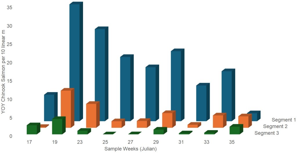
The overall counts of YOY Chinook salmon peaked in early May (Table 2). This may reflect that the study period may or may not have been reflective of actual peak abundance. U.S. Fish and Wildlife Service rotary screw trapping at Red Bluff Diversion Dam suggest that fall-run emergence and peak abundance occurs prior to the study period (Poytress 2014). The trend over time indicates that each run (fall-run, late fall-run and winter-run) appeared in the samples near their expected time of emergence and each race appeared to be represented throughout the sampling period. Only one YOY Chinook salmon was observed during the sampling of the river channel away from the banks. Throughout the study period, mesohabitats in the upper segment (Segment 1) had more YOY Chinook salmon residing in them than those in segment 2 (Fig. 3). Mesohabitats in the third segment were infrequently occupied by rearing fish. In-river mesohabitats (riffles, runs, pools, and glides) had an average of 10 YOY/10 linear m, while off-channel areas only had an average of two YOY per 10 linear m. Off-channel areas are defined as low elevation portions of the floodplain that are permanently inundated and permanently connected to the main river channel. Off-channel areas do not include side channels or connected or disconnected pools. Most of the off-channel areas were back-water coves.

Overall, there were significant differences in the proportion of occupied cells (Table 3) between the fourteen different cover types (C = 237.9, df = 535, P < 0.001). There was no significant difference in the proportion of occupied cells for complex woody cover types 4 (branches), 7 (overhead), 3.7 (fine woody + overhead), 4.7 (branches + overhead), 5.7 (log + overhead) and 9.7 (aquatic veg + overhead) (C = 6.68, df = 544, P = 0.25). Similarly, there was no significant difference in the proportion of occupied cells for the remaining eight (0 (no cover), 1 (cobble), 2 (boulder), 3 (fine woody), 5 (log), 8 (undercut bank), 9(aquatic veg), 10 (riprap)) cover types (C = 8.52, df = 542, P = 0.29). Based on this result, we defined two conglomerate cover categories, cover category 1, which included cover types 4, 7, 3.7, 4.7, 5.7 and 9.7, and cover category 2, which included the other eight cover types. There was a significant difference in the proportion of occupied cells for our conglomerate cover categories 1 and 2 (C = 221.9, df = 549, P < 0.001). Overall, the cover types were binned because there were not significant differences within the bins but there were significant differences between the bins.

For the site-level analysis, a model with percent cover category 1 had the best fit to the data, as compared to the full model (Table 4), with an AIC score of 26,195. This model had significant effects of cover (P < 0.001) for both the count model and the zero hurdle model. In contrast, a model with mesohabitat had the worst fit to the data, with an AIC score of 29,007, and a model with in-channel versus off-channel had a better fit to the data than the model with mesohabitat type. For the cell-level analysis, a model with cover category had the best fit to the data, as compared to the full model (Table 5), with an AIC score of 35,014. This model had significant effects of cover (P < 0.001) for both the count model and the zero hurdle model. In contrast, a model with mesohabitat had the worst fit to the data, with an AIC score of 36,880, and a model with in-channel versus off-channel had a better fit to the data than the model with mesohabitat type.

Table 4. AIC Scores of site-level models. First row is full model. (DOF = degrees of freedom)

Independent Variables	AIC Score	DOF
% Cover Category 1, Bank, Simplified Mesohabitat Type, Week, Segment, Week * Segment	25,429	66
% Cover Category 1, Bank, In-channel/off-channel, Week, Segment, Week * Segment	26,046	60
% Cover Category 1, Bank, Week, Segment, Week * Segment	26,195	58
Bank, Simplified Mesohabitat Type, Week, Segment, Week * Segment	29,007	64

Table 5. AIC Scores of cell-level models. First row is full model. (DOF = degrees of freedom)

Independent Variables	AIC Score	DOF
Cover Category, Bank, Simplified Mesohabitat Type, Week, Segment, Week * Segment	34,953	20
Cover Category, Bank, In-channel/Off-channel, Week, Segment, Week * Segment	35,078	14
Cover Category, Bank, Week, Segment, Week * Segment	35,132	12
Bank, Simplified Mesohabitat Type, Week, Segment, Week * Segment	36,880	18

Discussion

The temporal patterns in YOY abundance reflect the relative abundance and timing of the three runs of Chinook salmon. Fall-run, which spawn in October through December, followed by three months prior to emergence (Killam 2023), would be expected to have peak YOY abundance in the early portion of the sampling period, with numbers dropping over time due to mortality and outmigration. The peak in the smallest YOY size class we observed during the study period in late August likely reflects the newly emerging winter-run as a result of spawning in April through August. Spatial patterns of YOY at the segment scale reflect the distribution of spawning, with a majority of spawning for all three runs in Segment 1, and behavior of newly emerged YOY, moving short distances until they find suitable habitat conditions.

The lack of effect of mesohabitat type, with the exception of off-channel areas, reflects the large size and microhabitat diversity of mesohabitat units in the Sacramento River. Unlike smaller streams, the mesohabitat units in larger rivers have a wide range of depths and velocities, with wide overlap in microhabitat conditions between different mesohabitat types. In smaller streams, there is a close correlation between microhabitat and mesohabitat depths and velocities, making it impossible to separate out effects on YOY abundance of these two spatial scales. Larger rivers, in contrast, provide the opportunity to test the relative importance of these two spatial scales. The importance of the microhabitat scale, as shown in this study, is consistent with Railsback and Harvey (2011), which found that habitat use was driven by microhabitat scale processes (bioenergetics and predator avoidance).

The low YOY abundance in off-channel areas likely reflects other processes, such as impaired water quality and higher abundance of predators in off-channel versus riverine areas; future studies are recommended to test this hypothesis. No predators were seen during any of the surveys. In coastal streams, off-channel areas are important habitat features for juvenile coho salmon (Oncorhynchus kisutch), providing refugia from high in-channel velocities during winter high flows (Groot and Margulis 1991; Sandercock 1991; Nickelson et al. 1992; Lestelle 2007). In contrast, large highly regulated streams like the Sacramento River typically have a reversed flow regime, with the highest flows during the summer, negating the need for winter high flow refugia. Also, even at the lowest flows most of the Sacramento River, apart from near the banks, has velocities that are too high for juvenile salmonids. With changes in flow, the habitat zone for juvenile salmonids moves up the bank, and thus there is still habitat available even at higher flows.

The effects of depth and velocity could not be assessed in this study because of the wide range of depths and velocities within study sites and cells. Subsequent studies on the Sacramento River (Gard 2023) developed YOY Chinook salmon microhabitat suitability criteria for depth, velocity and cover, with the combination of the three variables best explaining YOY habitat use. The findings of this study are consistent with current knowledge of the Sacramento River, particularly the importance of cover as an aspect of YOY habitat.

Boone et al. (2012) showed the effectiveness of a statistical model that simultaneously evaluates both presence/absence and abundance for data with large numbers of zero values. The hurdle model used in this study uses a similar technique to that in Boone et al. (2012) with less assumptions. The hurdle model demonstrated that both presence/absence and abundance of YOY Chinook salmon is strongly influenced by the abundance of woody cover, since models including cover were the best models, compared to the full model, at both the site and cell scales.

Caveats regarding the limitations of this study include: 1) not all habitats within the river could be sampled because of turbidity, fast moving water, or deep water; and 2) this study was conducted in one river, over one season, in the spring. Different water years may produce environmental conditions and different results.

Management recommendations include: 1) habitat for large rivers should be assessed using microhabitat and not mesohabitat scales; 2) addition of woody cover should be included as part of restoration actions; and 3) for large, regulated rivers, off-channel areas should not be a focus of restoration actions.

Acknowledgements

Mention of specific products does not constitute endorsement by the U.S. Fish and Wildlife Service. We thank Larry Hanson and John Ferguson of the California Department of Fish and Wildlife and Jeff Thomas, Rick Williams and Paul Zedonis of the U.S. Fish and Wildlife Service for assistance with the fieldwork for this study. The study was funded by the Anadromous Fisheries Restoration Program (Section 3406[b][1]) of the Central Valley Project Improvement Act (Title XXXIV of P.L. 102-575).

Literature Cited

• Allouche, S. 2002. Nature and function of cover for riverine fish. Bulletin Français de la Peche et de la Pisciculture. 365/366:297–324.
• Bisson, P. A., K. Sullivan, and J. L. Nielsen. 1988. Channel hydraulics, habitat use, and body form of juvenile coho salmon, steelhead, and cutthroat trout in streams. Transactions of the American Fisheries Society 117:262–273.
• Boone, E. L., B. Steward-Koster, and M. J. Kennard. 2012. A hierarchical zero-inflated Poisson regression model for stream fish distribution and abundance. Environmetrics 23(3):207–218.
• Bovee, K. D., B. L. Lamb, J. M. Bartholow, C. B. Stalnaker, J. Taylor, and J. Henriksen. 1998. Stream habitat analysis using the instream flow incremental methodology. Information and Technology Report USGS/BRD-1998-0004.US Geological Survey, Biological Resources Division, Washington D.C., USA.
• California Department of Fish and Wildlife (CDFW). 1997. Central Valley anadromous fish-habitat evaluations, Sacramento and American river investigations, October 1995 through September 1996. Annual progress report prepared for U.S. Fish and Wildlife Service, Central Valley Anadromous Fish Restoration Program. Sacramento, CA, USA.
• Dietrich, W. E., and F. K. Ligon. 2009. RIPPLE: a digital terrain-based model for linking salmon population dynamics to channel networks. University of California, Berkeley and Stillwater Sciences, Berkeley, CA, USA. Available from: http://www.stillwatersci.com/resources/2009RIPPLEmodeloverview.pdf
• Fausch, K. D., C. E. Torgersen, C. V. Baxter, and H.W. Li. 2002. Landscapes to riverscapes: bridging the gap between research and conservation of stream fishes. A continuous view of the river is needed to understand how processes interacting among scales set the context for stream fishes and their habitat. BioScience 52(6):483–498.
• Gard, M. 2023. Central Valley anadromous salmonid habitat suitability criteria. California Fish and Wildlife Journal 109:e12.
• Groot, C. and L. Margolis. 1991. Pacific Salmon Life Histories. University of British Columbia Press, Vancouver, BC, Canada.
• Justice, C. 2007. Response of juvenile salmonids to placement of large woody debris in California coastal streams. Thesis, Humboldt State University, Arcata, CA, USA.
• Kemp, J. L., D. M. Harper, and G. A. Crosa. 2000. The habitat-scale ecohydraulics of rivers. Ecological Engineering 16(1):17–29.
• Killam, D. 2023. Salmonid populations of the upper Sacramento River basin in 2022. USRBFG Technical Report No. 02-2023. California Department of Fish and Wildlife, Red Bluff, CA, USA.
• Lestelle, L. C. 2007. Coho salmon (Oncorhynchus kisutch) life history patterns in the Pacific Northwest and California. Final report prepared for U.S. Bureau of Reclamation, Klamath Area Office, Klamath Falls, OR, USA.
• Naiman, R. J., and H. Decamps. 1997. The ecology of interfaces: riparian zones. Annual Review of Ecology and Systematics. 28:621–658.
• Nickelson, T. E., J. D. Rodgers, S. L. Johson, and M. F. Solazzi. 1992. Seasonal changes in habitat use by juvenile coho salmon (Oncorhynchus kisutch) in Oregon coastal streams. Canadian Journal of Fisheries and Aquatic Sciences 49(4):783–789.
• Parasiewicz, P. 2007. The MESOHABSIM model revisited. River Research and Applications 23(8):893–903.
• Poytress, W. R., J. J. Gruber, F. D. Carrillo, and S. D. Voss. 2014. Compendium report of Red Bluff Diversion Dam rotary trap juvenile anadromous fish production indices for years 2002–2012. U.S. Fish and Wildlife Service, Red Bluff, CA, USA.
• Pusey, B. J., and A. H. Arthington. 2003. Importance of the riparian zone to the conservation and management of freshwater fish: a review. Marine Freshwater Research. 54(1):1–16.
• Railsback, S. F., and B. C. Harvey. 2011. Importance of fish behaviour in modelling conservation problems: food limitation as an example. Journal of Fish Biology 79(6):1648–1662.
• Reeves, G. H., J. D. Sleeper, and D. W. Lang. 2011. Seasonal changes in habitat availability and the distribution and abundance of salmonids along a stream gradient from headwaters to mouth in coastal Oregon. Transactions of the American Fisheries Society 140:537–548.
• Sabal, M., S. Hayes, J. E. Merz, and J. D. Setka. 2016. Habitat alterations and a nonnative predator, the striped bass, increase native Chinook salmon mortality in the Central Valley, California. North American Journal of Fisheries Management 36(2):309–320.
• Sandercock, F. K. 1991. Life history of coho salmon, Oncorhynchus kisutch. Pages 395–446 inC. Groot and L. Margulis editors. Pacific Salmon Life Histories. University of British Columbia Press, Vancouver, BC, Canada.
• Snider, W. M., D. B. Christophel, B. L. Jackson, and P. M. Bratovich. 1992. Habitat characterization of the Lower American River. California Department of Fish and Wildlife, Sacramento, CA, USA.
• Steel, R. G. D., and J. H. Torrie. 1980. Principles and Procedures of Statistics. Second Edition. McGraw-Hill Book Company, New York, NY, USA.
• Welcomme, R. L. 1979. Fisheries Ecology of Floodplain Rivers. Longman, London, UK.
• Zeileis, A., C. Kleiber, and S. Jackman. 2008. Regression models for count data in R. Journal of Statistical Software 27(8):1–25.