

The findings and conclusions in this article are those of the author and do not necessarily represent the views of the U.S. Fish and Wildlife Service. This paper was prepared under the auspices of the U.S. Government and is therefore not subject to copywrite.
FULL RESEARCH ARTICLE
Mark Gard*
California Department of Fish and Wildlife, Conservation Engineering Branch, 1010 Riverside Parkway, West Sacramento, CA 95605, USA ![]() https://orcid.org/0009-0002-4529-9707
https://orcid.org/0009-0002-4529-9707
*Corresponding Author: mark.gard@wildlife.ca.gov
Published 21 Nov 2023 • doi.org/10.51492/cfwj.109.14
Abstract
Community-based macroinvertebrate habitat suitability criteria are needed for two reasons: (1) community-based criteria, such as with macroinvertebrates, are a better measure of ecosystem health than single-species habitat suitability criteria (HSC); and (2) if food rather than physical habitat is the limiting factor for juvenile salmonids, it is better to evaluate habitat restoration projects based on macroinvertebrate habitat than juvenile habitat. The goal of this study was to generate habitat suitability criteria for macroinvertebrates in the Sacramento River. Habitat suitability criteria were derived for three macroinvertebrate community metrics. One of the metrics (biomass of baetids, chironomids and hydropsychids) was selected to represent food supply for juvenile salmonids, while the other two metrics (total biomass and diversity) were selected as measures of ecosystem health. Baetidae, Chironomidae and Hydropsychidae were chosen because they are the dominant taxa present in stomach contents samples of Sacramento River juvenile Chinook Salmon Oncorhynchus tschawytscha. Habitat suitability criteria were developed using data from 75 macroinvertebrate samples stratified by season, mesohabitat type, depth, velocity, and substrate. The criteria for depth, velocity and substrate were developed taking into account several potential confounding variables, and using a polynomial regression for depth and velocity, and analysis of variance for substrate (a categorical variable). The criteria showed no effect of substrate on baetid/chironomid/hydropsychid biomass or diversity. Criteria for total biomass showed a higher suitability for larger cobbles, versus other substrates, for total biomass. The optimum depths for baetid/chironomid/hydropsychid biomass, total biomass and diversity were, respectively, 0.82–0.85 m, 0.61–0.67 m and 1.16–1.19 m. The optimum velocities for baetid/chironomid/hydropsychid biomass, total biomass and diversity were, respectively, 0.73–0.79 m/sec, 0.61–0.67 m/sec, and 0.61–0.73 m/s. Suggestions for development of future macroinvertebrate HSC include: (1) stratifying sampling by depth, velocity and substrate; (2) measuring the amount of organic matter in samples for use as an additional potential confounding factor; and (3) sampling a large area (0.84 m2) with a sampler with a rubber foam lining on the bottom of the sampler.
Key words: habitat suitability criteria, juvenile salmonids, macroinvertebrate, restoration, riverine
| Citation: Gard, M. 2023. Development of habitat suitability criteria for macroinvertebrate community metrics for use in habitat restoration projects. California Fish and Wildlife Journal 109:e14. |
| Editor: Lauren Miele, Habitat Conservation Planning Branch |
| Submitted: 4 May 2023; Accepted: 10 October 2023 |
| Copyright: ©2023, Gard. This is an open access article and is considered public domain. Users have the right to read, download, copy, distribute, print, search, or link to the full texts of articles in this journal, crawl them for indexing, pass them as data to software, or use them for any other lawful purpose, provided the authors and the California Department of Fish and Wildlife are acknowledged. |
| Funding: This study was funded by the Central Valley Project Improvement Act (Title XXXIV of P.L.102-575). |
| Competing Interests: The author has not declared any competing interests. |
Introduction
The intent of this paper is to present macroinvertebrate (generally the aquatic forms of insects) HSC that can be used to design and evaluate riverine habitat restoration projects. Habitat suitability criteria are used in habitat modeling to translate hydraulic and structural elements of rivers into indices of habitat quality (Bovee 1986; Bondi et al. 2013; Holmes et al. 2014; Gard 2023). Habitat suitability index (HSI), with values ranging from 0 to 1, is the response variable for HSC. Macroinvertebrate HSC have been developed previously (Gore et al. 2001; Holmquist and Waddle 2013; Waddle and Holmquist 2013); however, most of the previous macroinvertebrate HSC have been developed for individual taxa, including blackflies (family Simulidae), single gill mayflies (Deleatidium spp.), mayflies (family Ephemeroptera), stoneflies (family Plecoptera) and caddisflies (family Trichoptera) (Morin et al. 1986; Jowett et al. 1991; Wills et al. 2006). Choosing curves for individual taxa can be problematic when there are many species with different flow-habitat relationships as it is unclear how to select a single curve. Gore et al. (2001), Szalkiewicz et al. (2022), and Theodoropoulos et al. (2018) developed HSC for macroinvertebrate community diversity, with Gore et al. (2001) noting that the evaluation of macroinvertebrate communities is warranted because of the critical role of aquatic invertebrates in the processing of nutrients and organic energy in lotic systems and the increased emphasis on multi-species conservation. Gore et al. (2001) found that the bottleneck for fish populations in a North Carolina stream was macroinvertebrate habitat, rather than fish habitat. Community-based macroinvertebrate HSC are needed for two reasons: (1) community-based criteria, such as with macroinvertebrates, are a better measure of ecosystem health than single-species HSC because they integrate the habitat requirements of multiple species (Szalkiewicz et al. 2022; Theodoropoulos et al. 2018); and (2) given uncertainty in whether food or physical habitat is the limiting factor for juvenile salmonids, it is advisable to evaluate habitat restoration projects based on both macroinvertebrate and juvenile habitat (Gore et al. 2001). More macroinvertebrate habitat can result in higher energy flow potential for juvenile salmon feeding on macroinvertebrates, which can increase growth rates, and thus can result in higher survival when reaching salt water.
The goal of this study was to generate HSC for macroinvertebrates in the Sacramento River between Keswick Reservoir and Battle Creek. Macroinvertebrates were selected as a measure of food abundance for juvenile salmonids (Gore et al. 2001), as well as an indicator of ecosystem health, per Szalkiewicz et al. (2022) and Theodoropoulos et al. (2018).
Methods
Sampling
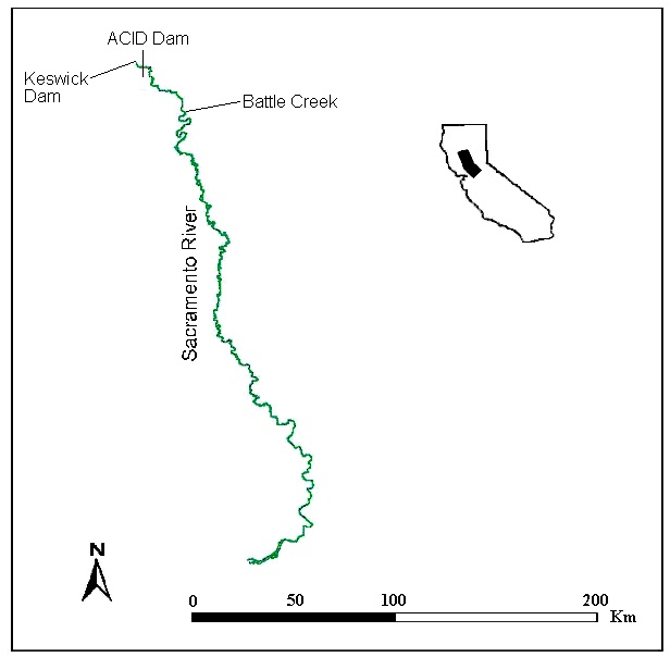
Macroinvertebrate samples were collected from the Sacramento River, California between Anderson-Cottonwood Irrigation District Dam (122˚23’38”W, 40˚35’32”N) and Battle Creek (122˚10’33”W, 40˚21’18”N, Fig. 1), with sampling locations randomly selected. Samples were collected in this reach because it is the focus of Sacramento River habitat restoration projects. Elevations range from 110–145 m, while Sacramento River flows are typically between 92–425 m3/s. The study area has a Mediterranean climate, with most rainfall in November through May. The Sacramento River is dominated by a cold-water fish assemblage, including Chinook Salmon (Oncorhynchus tschawytscha) and steelhead (Oncorhynchus mykiss). The Sacramento River has four runs of Chinook Salmon (fall, late-fall, spring, and winter), with the name corresponding to the timing of freshwater entry. After freshwater entry, adult anadromous salmonids spawn, creating redds. After several months, fry emerge from the redds and rear in freshwater from several months to over a year before emigrating to the ocean. The collection of macroinvertebrate data began in July 1999 and was completed in January 2001. To eliminate potential effects on the macroinvertebrate population due to changes in flow, the goal was to have at least 30 days of stable discharge from Keswick Dam prior to sample collection. Samples could not be collected from August to October 1999, December 1999 to July 2000, and from September to October 2000 due to varying flows. Stable discharges ensured that macroinvertebrate community composition reflected the conditions (depths and velocities) present during sampling.
The sampling plan included stratifying sampling by season, mesohabitat type, depth, velocity and substrate. Frequent fluctuations of Keswick Dam releases during most of the year typically only left two periods which had relatively constant flows for 30 days: mid-summer, usually starting around early July; and mid-fall, generally starting around early October. Thus, the only times suitable for sampling were typically in mid-August and mid-November. However, relatively constant flows from Keswick Dam extended into the winter of 2000–2001, allowing additional sampling to occur in December 2000 and January 2001. Sampling sites selected based on the above stratification protocol were identified with a weighted tag placed at the sampling location. Before a sample was collected, the depth and mean column velocity at the sampling site were measured and the substrate size was noted (Table 1).
Table 1. Substrate codes, descriptors, and particle sizes from Gard (2006).
| Code | Type | Particle size (cm) |
| 0.1 | Sand/Silt | < 0.25 |
| 1 | Small Gravel | 0.25–2.5 |
| 1.2 | Medium Gravel | 2.5–5 |
| 1.3 | Medium/Large Gravel | 2.5–7.5 |
| 2.3 | Large Gravel | 5–7.5 |
| 2.4 | Gravel/Cobble | 5–10 |
| 3.4 | Small Cobble | 7.5–10 |
| 3.5 | Small Cobble | 7.5–12.5 |
| 4.6 | Medium Cobble | 10–15 |
| 6.8 | Large Cobble | 15–20 |
| 8 | Large Cobble | 20–25 |
| 9 | Boulder/Bedrock | > 30 |
| 10 | Large Cobble | 25–30 |
A customized macroinvertebrate Surber sampler was constructed to use in this effort. The sampler was used to collect macroinvertebrates from a 0.84 m2 area. The sampler was 1.22 m high, so it could be used to sample areas with depths up to 1.22 m. The sampler consisted of a steel-rod frame with fine-mesh seine material on the sides and brackets for a detachable net on the back. The net had a 0.91 x 1.22 m opening, a mesh size of 600 μm, and was mounted on a rectangular 0.91 x 1.22 m steel frame. The bottom of the sampler had a rubber foam lining to provide a tight seal with the substrate when the sampler was pressed down to the river bottom. The sampler required three individuals: typically, one to hold the sampler in place, and the other two individuals to clean off rocks within the 0.84 m2 area, with the current carrying the macroinvertebrates into the net. Sites less than 0.91 m deep were sampled by two individuals with snorkel gear, while sites over 0.91 m deep were sampled by one individual with SCUBA gear. In the latter case, two individuals held the sampler in place. Rocks were cleaned to a depth below the channel bottom of 0.1–0.15 m. Bedrock was cleaned with a 0.08 x 0.15 m scrub brush, while rocks were picked up and cleaned underwater by rubbing with neoprene gloves. After sampling was completed, the net was detached from the sampler, the macroinvertebrates in the net were washed into the cod end of the net and then transferred to jars with 70% alcohol for transport back to the lab for analysis.
Processing
U.S. Fish and Wildlife Service (USFWS) staff conducted the initial processing of one third of the samples, separating macroinvertebrates from detritus. The initial processing of the remaining two thirds of the samples and final processing of all of the samples, including sorting, identification and enumeration of taxa and measurement of biomass (ash-free dry weight) of Baetidae, Chironomidae, Hydropsychidae, and all remaining taxa, was conducted by Environmental Services and Consulting, LLC (ESC), under contract to the USFWS. Three metrics for the macroinvertebrate data were developed to use in deriving HSC: (1) Shannon Diversity Index (diversity, Spellerberg and Fedor 2003); (2) combined ash-free dry weight (AFDW) of Baetidae, Chironomidae, and Hydropsychidae (BCH); and (3) total AFDW of macroinvertebrates. Baetidae, Chironomidae and Hydropsychidae were chosen because they are the dominant taxa present in stomach contents samples of Sacramento River juvenile Chinook Salmon Oncorhynchus tschawytscha (Saiki et al. 2001). Diversity and total AFDW, common macroinvertebrate metrics, were selected as indicators of ecosystem health (Szalkiewicz et al. 2022; Theodoropoulos et al. 2018).
Analyses
An assumption of this study is that invertebrates adjust to flows in 30 days, per Harvey (1986). The study tests a series of hypotheses that invertebrates may be affected by season (early July and mid-fall), mesohabitat type, sample assessor (USFWS versus ESC), depth, velocity, and substrate. The first step in developing the HSC was to determine if there were significant correlations between depth, velocity, and substrate size. Kolmogorov-Smirnov one-sample tests (SYSTAT 2002) were then used to determine if diversity, BCH AFDW and total AFDW were normally distributed or if they could be transformed to be normally distributed via a logarithmic or square root transformation.
Three potentially confounding categorical variables were identified: (1) sample assessor (whether samples had been initially processed by USFWS staff or by ESC); (2) mesohabitat type (with four levels: riffle, run, pool or glide); and (3) sampling event (with four levels: July 1999, November 1999, August 2000, and November 2000–January 2001). These potentially confounding categorical variables were identified because there was variation among the data in them, and they could plausibly have an effect on the macroinvertebrate metrics. Kruskal-Wallis One-Way Analysis of Variance (SYSTAT 2002) was used to test if these confounding variables had a significant effect on diversity, BCH AFDW and total AFDW. In cases where there was a significant effect of one or more confounding variables on a HSC metric, a generalized linear mixed effects model (SYSTAT 2002) with fixed and random effects was tested with terms consisting of: (1) the confounding categorical variable(s) (fixed effect) and V, V 2, V 3 and V 4, where V is velocity or depth (continuous variable, random effect); or (2) the confounding categorical variable(s) and substrate code (as a categorical variable). If there was no significant effect of the confounding variable(s) in the generalized linear mixed effect model, the confounding variable(s) were dropped from the analysis. In these cases, substrate HSC were developed for each macroinvertebrate metric using one-way analysis of variance (SYSTAT 2002), or t-tests where the substrate categories were merged into two groups. The latter case was used where the generalized linear mixed effect model did not show a significant effect of substrate, but the data showed two groups of substrate codes where there might be a significant difference between the groups but no significant difference within each group.
For cases in which the confounding variable(s) were dropped from the analysis, depth and velocity HSC for each macroinvertebrate metric were derived using a polynomial regression (SYSTAT 2002), with dependent variable diversity, BCH AFDW or total AFDW, and independent variable depth or velocity. The regression fit the data to the following expression:
Metric = I + J V + KV2 + LV3 + MV4
where metric was diversity, BCH AFDW or total AFDW; I, J, K, L, and M are coefficients calculated by the regression; and V is velocity or depth. The regressions were conducted in a sequential fashion, where the first regression tried was a fourth order regression with all terms. If any of the coefficients or the constant were not statistically significant at p = 0.05, the term with the highest p value was dropped from the regression equation, and the regression was repeated, until a regression was arrived at for which all terms had p < 0.05. An a priori hypothesis for the depth regressions was that the HSI for a depth of zero should be zero. As a result, a constant term was not used in the depth regressions. This is a standard approach used in developing HSC (Gard 2023), where the goal is to generate the best fit of the HSC function to the underlying data. Where the confounding variable(s) were significant in the generalized linear mixed effect model, depth and velocity HSC were derived using the depth and velocity coefficients from the generalized linear mixed effect model. The results of the regression equations were rescaled so that the highest value was 1.0 and were truncated at the upper end where the value of the regression reached zero.
Results
Sampling
A total of 75 macroinvertebrate samples were collected (Table 2). A typical assumption is that at least 150 samples are needed to develop HSC (Bovee 1986). Given the stratification of the sampling by depth, velocity, and substrate, I concluded that the 75 samples collected were sufficient to generate HSC. Stratifying by depth, velocity and substrate allows for a smaller sample size because the variation in the data attributable to each independent variable can be separated. Of these samples, 22 were collected in riffles, 20 in runs, 13 in pools and 20 in glides. Water depths of the samples ranged from 0.24 to 1.31 m, while the velocities of the samples ranged from 0.122 to 1.481 m/s. Samples were collected for the entire range of substrate types in Gard (2006), ranging from sand/silt to bedrock.
Table 2. Macroinvertebrate Habitat Suitability Criteria sampling dates, Sacramento River flows, and number of samples.
| Sampling dates | Keswick release during sampling (m3/s) | Keswick release for 30 days prior to sampling (m3/s) | # samples |
| 26–28 July 1999 | 371.9 | 378.7 ± 5% | 10 |
| 16 Nov 1999 | 178.4 | 175.0 ± 3% | 6 |
| 1–4 Aug 2000 | 426.2 | 421.0 ± 6% | 19 |
| 7 Aug 2000 | 402.1 | 421.0 ± 6% | 2 |
| 28–30 Nov 2000 | 170.6 | 153.4 ± 18% | 14 |
| 4–6 Dec 2000 | 161.3 | 153.1 ± 6% | 12 |
| 16–18 Jan 2001 | 123.4 | 124.3 ± 9% | 12 |
Analyses
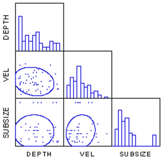
A correlation analysis (SYSTAT 2002) indicated that there were no significant (P > 0.1) correlations between depth, velocity, and substrate size (Fig. 2). Kolmogorov-Smirnov one sample tests (SYSTAT 2002) indicated that diversity, BCH AFDW and total AFDW were not normally distributed (P < 0.01), nor would they be normally distributed with a logarithmic or square root transformation (P < 0.01). No non-parametric alternatives exist, so I proceeded on the assumption that the analyses were robust enough to handle this violation of assumptions.
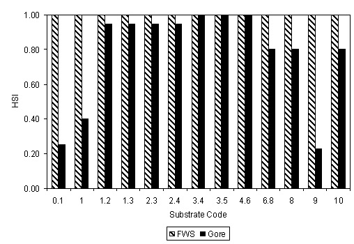
There were significant effects of sample assessor on BCH AFDW and diversity, and of sampling event on total AFDW and diversity (P < 0.05, Kruskal-Wallis One-Way Analysis of Variance [SYSTAT 2002]) (Table 3). In contrast, there was no significant effect at P = 0.05 of sample assessor on total AFDW, of sampling event on BCH AFDW, or of mesohabitat type on any of the three macroinvertebrate metrics. For BCH AFDW versus depth, velocity and substrate, there was no significant effect of sample assessor (P > 0.13, generalized linear mixed effect model (SYSTAT 2002)), and thus sample assessor was dropped from the analysis. The generalized linear mixed effect model for substrate did not show a significant effect of substrate (P = 0.66). For total AFDW versus depth, velocity and substrate, there was no significant effect of sampling event (P > 0.125, generalized linear mixed effect model (SYSTAT 2002)), and thus sampling event was dropped from the analysis. The generalized linear mixed effect model for substrate did not show a significant effect of substrate (P = 0.46), nor did a one-way analysis of variance (P = 0.48). There appeared to be a difference in total AFDW between larger substrates (substrate codes 6.8, 8 and 10) and smaller substrates and bedrock. A two-sample t-test showed a significant difference between larger (mean = 2.76 g) and smaller substrates (mean = 0.74 grams, P = 0.039), as did a generalized linear mixed effect model with sample week and the above two levels of substrate (P = 0.01). The effect of sampling event was not significant (P = 0.36) in this generalized linear mixed effect model. As a result, the initial total AFDW suitability was 2.76 for substrate codes 6.8, 8, and 10, and 0.74 for all other substrate codes. These initial values were rescaled so that the largest suitability was 1 (Fig. 3).
Table 3. Results of statistical tests for effects of confounding variables. Y = significant effect at P = 0.05, N = no significant effect at P = 0.05, N/A = not applicable (when N for metric versus confounding variable).
| Metric/Independent Variable | Mesohabitat Type | Sampling Event | Sample Assessor |
| Diversity | N | Y | Y |
| BCH | N | N | Y |
| Total AFDW | N | Y | N |
| Diversity/Depth | N/A | Y | N |
| Diversity/Velocity | N/A | Y | N |
| Diversity/Substrate | N/A | Y | N |
| BCH/Depth | N/A | N/A | N |
| BCH/Velocity | N/A | N/A | N |
| BCH/Substrate | N/A | N/A | N |
| Total AFDW/Depth | N/A | N | N/A |
| Total AFDW/Velocity | N/A | N | N/A |
| Total AFDW/Substrate | N/A | N | N/A |

For diversity versus depth, velocity and substrate, there was no significant effect of sample assessor (P > 0.54, generalized linear mixed effect model [SYSTAT 2002]), and thus sample assessor was dropped from the analysis. However, there was a significant effect of sampling event (P < 0.0009) for all three variables. The generalized linear mixed effect model for substrate did not show a significant effect of substrate (P = 0.45), nor did there appear to be any significant differences in diversity between substrate codes. A Kruskal-Wallis one-way analysis of variance (SYSTAT 2002) also did not show a significant difference in diversity between substrates (P = 0.42).
Sampling event was incorporated into the subsequent development of depth and velocity HSC for diversity using the depth and velocity coefficients from the generalized linear mixed effect model. For diversity versus depth, the p values for all depth terms were greater than 0.05. As a result, the final criteria for diversity had a suitability of 1 for all depths except 0, which had a suitability of 0. The coefficients for the final regressions for depth and velocity for each macroinvertebrate metric are shown in Table 4.
Table 4. Coefficients for the final regressions for depth and velocity (V) for each Sacramento River macroinvertebrate metric. The P-values for all of the non-zero coefficients were less than 0.05, as were the P-values for the overall regressions. The only exception to this was the V2 term for baetid/chironomid hydropsychid ash free dry weight (BCH AFDW), with a P-value of 0.058. This term was retained even though its P-value was greater than 0.05 because the regression would be biologically unrealistic (continually increasing HSI with velocity) with only the V term. I is the constant and J, K, L and M are the regression coefficients in equation (1). A coefficient or constant value of zero indicates that term or the constant was not used in the linear regression, because the P value for that coefficient or for the constant was greater than 0.05.
| Metric | Parameter | I | J | K | L | M | R2 |
| BCH AFDW | depth | 0 | 0 | 0.1614 | –0.0393 | 0 | 0.24 |
| BCH AFDW | velocity | 0 | 0.2588 | –0.0517 | 0 | 0 | 0.23 |
| total AFDW | depth | 0 | 1.87 | –0.4366 | 0 | 0 | 0.20 |
| total AFDW | velocity | 0 | 1.726 | –0.3914 | 0 | 0 | 0.19 |
| diversity | velocity | 1.5606 | 0 | 0.38771 | –0.18187 | 0.02175 | 0.37 |
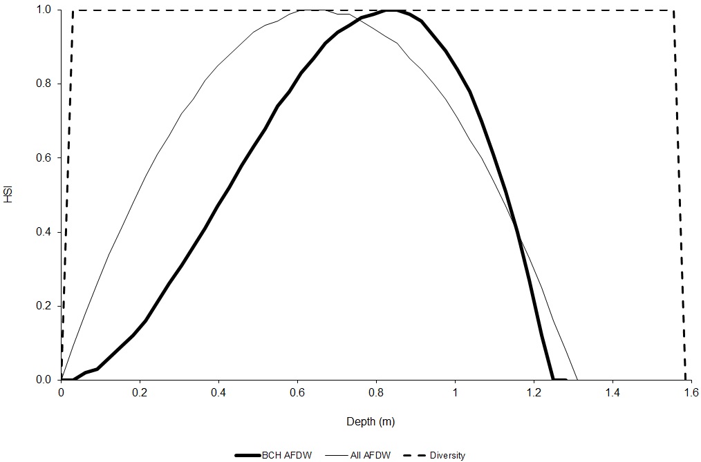
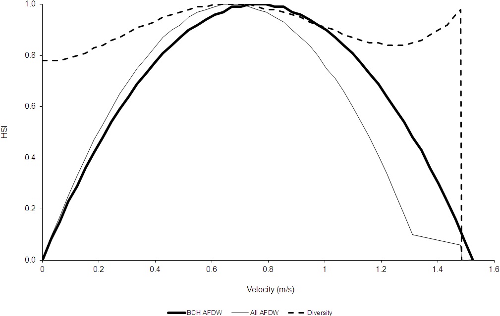
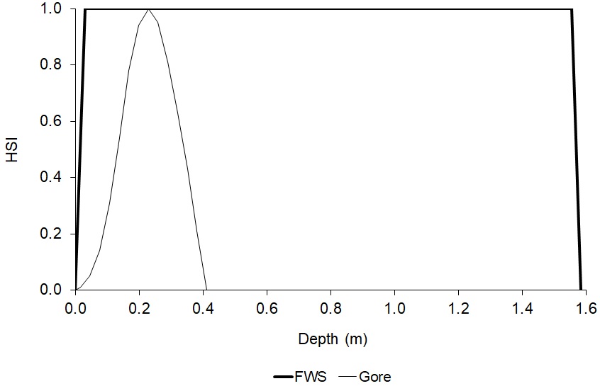
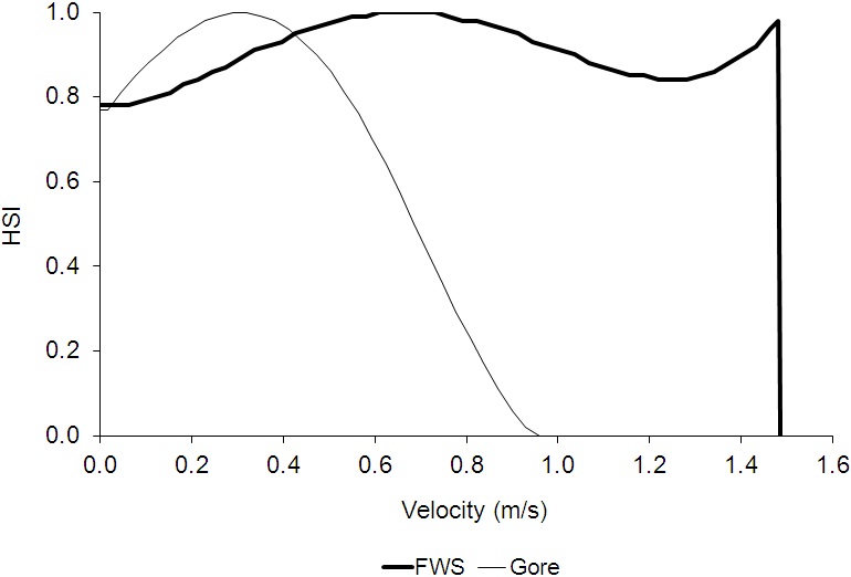
For total AFDW versus velocity, the regression equation predicted that total AFDW would become negative at values less than the largest sampled velocity, even though there was a non-zero measured total AFDW at this value (1.481 m/s). In this case, I stopped using the regression at the highest velocity which had a predicted total AFDW greater than zero (1.31 m/s), then calculated a HSI value for 1.481 m/s by dividing the total AFDW at 1.481 m/s (1.21 g) by the highest measured total AFDW (20.27 g) and set the suitability for velocities greater than 1.481 m/s to zero. For diversity versus velocity, the regression equation predicted that diversity would continually increase for velocities greater than the maximum sampled velocity (1.481 m/s). As a result, the regression was truncated at 1.481 m/s, setting the suitability for velocities greater than 1.481 m/s to zero. A general practice in developing HSC is to not extrapolate beyond the range of measured values (Gard 2023). The final depth and velocity criteria are shown in Figures 4 and 5.
Discussion
The macroinvertebrate HSC from this study can be used, together with hydraulic models, to develop flow-habitat relationships for existing and proposed conditions and thus document benefits of habitat restoration projects for macroinvertebrates. The optimum depth and velocity for macroinvertebrates are comparable to those for anadromous salmonid spawning (0.3–1 m, 0.3–1 m/s) (Gard 2023). The principal difference between macroinvertebrate and anadromous spawning habitat is the preference for cobbles for macroinvertebrates, versus gravel for spawning (Gard 2006). Incorporating up to 25% cobble into spawning gravel will benefit macroinvertebrate habitat while not adversely affecting spawning habitat. In fact, this change will ultimately benefit spawning habitat by slowing the loss of spawning gravels from habitat restoration sites due to mobilization of sediment at high flows (Zeug et al. 2014). In contrast, there is little overlap between macroinvertebrate habitat and juvenile salmonid physical habitat, which is generally slow, shallow with woody cover (Gard 2023).
Seasonal variations in macroinvertebrate diversity did not affect HSC derived from this study. By using the variable sampling event (with four levels: July 1999, November 1999, August 2000, and November 2000–January 2001) in my analysis, I was able to take into account responses of the macroinvertebrate community to changes in the amount of organic matter accumulated in the riverbed due to seasonal flood flows as well as changes in macroinvertebrate communities associated with seasonal effects on their life cycles. The above seasonal variations did not affect BCH AFDW since there was no significant effect of sampling event on this metric. Further, after depth, velocity and substrate were taken into account, there were no effects of sampling event on total AFDW. Thus, any apparent effects of seasonal variations on total AFDW were actually due to variations between sampling periods in the depths, velocities and substrates sampled. By including sampling event in the development of the HSC for diversity, I was able to determine the effects of depth, velocity and substrate that were independent of seasonal variations in macroinvertebrate diversity, and thus find that the HSC derived for diversity were not affected by seasonal variations in macroinvertebrate diversity. Put another way, the seasonal variations in macroinvertebrate diversity did not obscure nor did they cause the derived relationships between diversity and depth, velocity, and substrate.
Based on the following discussion, the hypotheses made in this study are valid. The linear models used in this study addressed the hypotheses that invertebrates are affected by season, mesohabitat and sample assessor by separating out the effects of these potentially confounding variables from the effects of depth, velocity and substrate on the macroinvertebrate metrics used in this study. Substrate disturbance history, driven by flow events and floods in particular, can affect biomass and species composition of macroinvertebrates (Gholizadeh 2021). However, in this case, sediment disturbance history did not affect the samples because samples were only collected when the flows were relatively constant for the 30 days prior to sampling (Table 2), ensuring that the depths and velocities present during data collection were similar to those present during macroinvertebrate colonization. I conclude that it is not necessary to take into account the duration of flooding/flow 45 or 60 days prior to sampling, based on Harvey’s (1986) findings that macroinvertebrates had completely recolonized areas below suction dredge mining areas within 45 days after the cessation of suction dredge mining; if macroinvertebrates can completely recolonize areas within 45 days, it is reasonable to expect that macroinvertebrate community characteristics would adjust to changes in depth and velocity within 30 days.
There are significant differences between the diversity of HSC from Gore et al. (2001) and those developed in this study (Figs. 6–8). For example, this study found that the maximum suitability for depth was at 1.16–1.19 m, whereas the Gore et al. (2001) criteria had a suitability for diversity that reached zero at a depth of 0.411 m. Further, this study found a relatively weak effect of depth, velocity, and substrate on diversity. It is likely that the differences between the HSC from this study and those from Gore et al. (2001) were because the HSC in this study were developed from samples taken from a single stream, which the HSC in Gore et al. (2001) were developed from samples taken from multiple streams. The results of this study indicate that biomass may be a better metric of macroinvertebrates than diversity for evaluating habitat restoration projects, although biomass does have some drawbacks, such as favoring larger-bodied species.
The lack of significant correlations between depth, velocity, and substrate size was expected, given the stratified sampling design. Since the generalized linear mixed effect models for BCH AFDW and diversity did not show a significant effect of substrate, I concluded that there was no significant effect of substrate for these two metrics and set the HSI value of these two metrics to 1.0 for all substrate codes.
This study shows the importance of stratifying macroinvertebrate samples by depth, velocity, and substrate, consistent with the findings of Dolodec et al. (2007), Kokes (2011), Sagnes et al. (2008), and Stazner et al. (1988, 1998). Without stratified sampling, there would be a tendency to get low suitabilities for large depths if all of the samples with large depths were collected in areas with low velocities, which would bias the depth criteria towards shallow depths. This study also demonstrates the need for a larger sampler when sampling large substrate sizes. With the usual 0.09 m2 sampler, only one large cobble would be sampled, which would be too small of a sample. Having a rubber foam lining on the bottom of the sampler is critically important, particularly for larger-sized substrates. Many of the invertebrates would be lost passing under the frame of a typical Surber sampler. The amount of organic matter in the samples was not measured. Future studies should measure the amount of organic matter in the samples to use as an additional potential confounding variable in developing macroinvertebrate HSC.
In conclusion, the HSC developed in this study can be used as one tool in designing habitat restoration projects, both within and outside of the study area. Additionally, the lessons learned from this study will be useful in informing future studies that are developing macroinvertebrate criteria for habitat suitability modeling.
Acknowledgements
I thank E. Ballard, E. Sauls, J. Big Eagle, B. Null, R. DeHaven, E. Irwin, L. Thompson, D. Buford and R. Williams for assistance with the fieldwork for this study. J. Big Eagle, L. Lewis and K. Turner conducted initial analysis of a third of the samples, separating macroinvertebrates from detritus. The remaining portion of the sample analysis was conducted by Environmental Services and Consulting, LLC. This study was funded by the Central Valley Project Improvement Act (Title XXXIV of P.L.102-575). Mention of specific products does not constitute endorsement by the U.S. Fish and Wildlife Service.
Literature Cited
- Bondi, C. A., S. M. Yarnell, and J. Lind. 2013. Transferability of habitat suitability criteria for a stream breeding frog (Rana boylii) in the Sierra Nevada, California. Herpetological Conservation and Biology 8(1):88–103.
- Bovee, K. D. 1986. Development and evaluation of habitat suitability criteria for use in the Instream Flow Incremental Methodology. Instream Flow Information Paper 21. Biological Report OBS-86/7, U. S. Fish and Wildlife Service, Washington, D.C., USA.
- Dolodec, S., N. Lamoroux, U. Fuchs, and S. Merigoux. 2007. Modelling the hydraulic preferences of benthic macroinvertebrates in small European streams. Freshwater Biology 52:145–164.
- Gard, M. 2006. Modeling changes in salmon spawning and rearing habitat associated with river channel restoration. International Journal of River Basin Management 4(3):201–211.
- Gard, M. 2023. Central Valley anadromous salmonid habitat suitability criteria. California Fish and Wildlife Journal 109:e12.
- Gholizadeh, M.2021. Effects of floods on macroinvertebrate communities in the Zarin Gol River of northern Iran: implications for water quality monitoring and biological assessment.Ecological Processes 10:46.
- Gore, J. A., J. B. Layzer, and J. Mead. 2001. Macroinvertebrate instream flow studies after 20 years: a role in stream management and restoration. Regulated Rivers: Research and Management 17:527–542.
- Harvey, B. C. 1986. Effects of suction gold dredging on fish and invertebrates in two California streams. North American Journal of Fisheries Management 6:401–409.
- Holmquist, J .G., and T. J. Waddle. 2013. Predicted macroinvertebrate response to water diversion from a montane stream using two-dimensional hydrodynamic models and zero flow approximation. Ecological Indicators 28:115–124.
- Holmes, R. W., M. A. Allen, and S. Bros-Seeman. 2014. Seasonal microhabitat selectivity by juvenile steelhead in a central California coastal river. California Fish and Game 100:590–615.
- Jowett, I. G., J. Richardson, B. J. F. Biggs, C.W. Hickey, and J. M. Quinn. 1991. Microhabitat preferences of benthic invertebrates and the development of generalized Deleatidium spp. habitat suitability curves, applied to four New Zealand rivers. New Zealand Journal of Marine and Freshwater Resources 25:187–199.
- Kokes, S. J. 2011. River channel habitat diversity (RCHD) and macroinvertebrate community. Versita Biologia 66:328–334.
- Morin, A., P-P. Harper, and R. H. Peters. 1986. Microhabitat-preference curves of blackfly larvae (Diptera: Simuliidae): a comparison on three estimation methods. Canadian Journal of Fisheries and Aquatic Science43:1235–1241.
- Saiki, M. K., B. A. Martin, L. D. Thompson, and D. Welsh. 2001. Copper, cadmium, and zinc concentrations in juvenile Chinook salmon and selected fish-forage organisms (aquatic insects) in the upper Sacramento River, California. Water, Air, and Soil Pollution 132:127–139.
- Sagnes, P. S., S. Merigoux, and N. Peru. 2008. Hydraulic habitat use with respect to body size of aquatic insect larvae: case of six species from a French Mediterranean stream. Limnologica 38:23–33.
- Spellerberg, I. F., and P. J. Fedor. 2003. A tribute to Claude Shannon (1916–2001) and a plea for more rigorous use of species richness, species diversity and the ‘Shannon-Wiener’ Index. Global Ecology and Biogeography 12(3):177–179.
- Stazner, B., J. A. Gore, and V. H. Resh. 1988. Hydraulic stream ecology: observed patterns and potential applications. Journal of the North American Benthological Society 7:307–360.
- Stazner, B., J. A. Gore, and V. H. Resh. 1998. Monte Carlo simulation of benthic macroinvertebrate populations: Estimates using random, stratified, and gradient sampling. Journal of the North American Benthological Society17:324–337.
- SYSTAT. 2002. SYSTAT 10.2 Statistical Software. SYSTAT Software Inc., Richmond, CA, USA.
- Szalkiewicz, E., T. Kaluza, and M. Grygoruk. 2022. Detailed analysis of habitat suitability curves for macroinvertebrates and functional feeding groups. Scientific Reports 12:10757.
- Theodoropoulos, C., A. Vourka, N. Skoulikidis, and P. Rutschmann. 2018. Evaluating the performance of habitat models for predicting the environmental flow requirements of benthic macroinvertebrates. Journal of Ecohydraulics 3(1):30–44.
- Waddle, T. J., and J. G. Holmquist. 2013. Macroinvertebrate response to flow changes in a subalpline stream: predictions from two-dimensional hydrodynamic models. River Research and Applications29:366–379.
- Wills, T. C., E. A. Baker, A. J. Nuhfer, and T. G. Zorn. 2006. Response of the benthic macroinvertebrate community in a northern Michigan stream to reduced summer streamflows. River Research and Applications22:819–836.
- Zeug, S. C., K. Sellheim, C. Watry, B. Rook, J. Hannon, J. Zimmerman, D. Cox, and J. Merz. 2014. Gravel augmentation increases spawning utilization by anadromous salmonids: a case study from California, USA. River Research and Applications 30(6):707–718.
Appendices for “Development of habitat suitability criteria for macroinvertebrate community metrics for use in habitat restoration projects”