FULL RESEARCH ARTICLE

Robert M. Sullivan*

Northern California Wildlife Ecology and Fisheries Sciences, Weaverville, CA 96093, USA

*Corresponding Author: robert.m.sullivan@icloud.com

Published 21 Nov 2023 • http://www.doi.org/10.51492/cfwj.109.13

Abstract

In resource management, the kind and extent of ecological co-occurrence between closely related species frequently requires assessment of the spatial relationship among taxa. In my study, analysis of inter-species pair-wise distances revealed no syntopic overlap between Church’s sideband (Monadenia churchi) and Trinity bristle snails (M. setosa). No pair of samples had the same geographic coordinates and no parapatric boundary in environmental covariates was evident between species. This “microsympatric” spatial relationship resembled a metapopulation structure with no high degree of overlap, as co-occurrence was rare and small in geographic scope. Fifteen forest cover-types and 82 soil-types were identified between species. The most common forest-type for M. churchi was Sierra Mixed Conifer (39.9%) and Douglas fir (28.9%). In M. setosa the most common forest-types were the same but in much different percentages (78.8% and 14.8%, respectively). Sixty-one and 39 soil-types were associated with samples of M. churchi and M. setosa, respectively. The Hohmann-Neuns family complex was the most common (22.5%) soil-type for M. churchi and the Holland Deep-Hugo family complex was the most (50.6%) dominant for M. setosa. There were significant differences between species in all environmental attributes and in values of monthly temperature and precipitation, which reflected variance in the mesoclimatic regime seasonally. Principal Components Analysis (PCA) accounted for 57.8% of the dispersion contained in environmental variables on the first 3-eigenvectors. Evapotranspiration and Summer and Winter Temperatures loaded positively while Summer and Winter Precipitation and Elevation loaded negatively along PC I (26.2%). Given significant inter-species differences in ecological occupancy, it seems plausible that microsympatry is based in part on both mesoscale habitat variance and subtle differences in mesoclimate defined by seasonal variation in temperature and precipitation. The hypothesis that M. setosa is adapted to cool habitats and M. churchi to warmer more arid environs in microsympatry was substantiated at a macroscale level.

Key words: co-occurrence, ecological assessment, land snail, microsympatric, Monadenia churchi, Monadenia setosa, sympatric, syntopic, temperature regime

Introduction

Sympatry is a term used to describe species that occur in the same place at the same time with overlapping geographic ranges. This relationship may include the same local community such that they are close enough to interact (i.e., microsympatry; Jorgensen and Fath 2008).

In contrast, parapatry describes a situation where geographically separated ranges of closely related species abut along a common boundary as a function of spatial changes in environmental factors (Anderson and Evensen 1978; Bull 1991; King 1993), which define species-specific habitats across their parapatric boundary. Alternatively, the term “syntopy” is used to describe individuals of different species that occur side-by-side in nature, using the same habitats. Historically, a primary goal of community ecology has focused on discerning what factors drive the distribution and associated spatial relationships of species that occur in both sympatry and allopatry. The study of sympatry, particularly in populations of closely related species (i.e., sister taxa), has contributed to many important and contentious ideas in ecology and evolutionary biology (Jorgensen and Fath 2008). Several factors may influence the ecological and spatial relationships among species. Such factors may include abiotic conditions and/or biotic interactions. Knowledge of how these factors influence the distribution of animal communities is central to understanding the ecological and spatial relationships among co-occurring taxa (Soberón 2007; Heart et al. 2018).

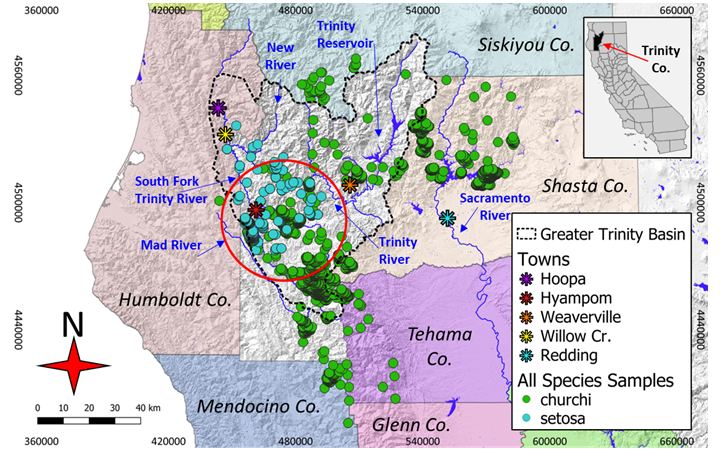
In northern California, terrestrial snails are widely distributed within forest and woodland ecosystems. Church’s sideband snail (Monadenia churchi) and the Trinity bristle snail (M. setosa) have coincident spatial distributions in a small area within the south-central portion of the Greater Trinity Basin (Fig. 1). The geographic distribution of M. setosa includes the Klamath Bioregion centered on the southwestern edge of the Greater Trinity Basin watershed (Sullivan 2021). In comparison, the range of M. churchi encompasses virtually the entire Greater Trinity Basin, including areas outside the basin south to the northern extent of North Coast Bioregion and east to the Sacramento River Valley at the edge of the Sierra Nevada escarpment (Fig. 1). Taxonomically, the geographic distribution of M. setosa lies on the eastern edge of the subgenus Monadenia, whereas the range of M. churchi belongs to the inland subgenus Shastelix (Roth 1981; Roth and Sadeghian 2006). These subgeneric relationships appear reflected in a recent phylogenetic analysis (Sullivan 2021) summarizing geographic variation within riverine-segregated populations of M. setosa, where M. churchi and M. mormonum (Sierra sideband) were hypothesized to be sister species to M. infumata subcarinate (Redwood sideband), M. ochromphalus (yellow-based sideband), and M. setosa.

Although co-occurrence and qualitative habitat differences between M. churchi and M. setosa were highlighted early on (Hanna and Smith 1933; Roth 1978), the ecological preference and degree to which these two taxa segregate spatially is yet unclear and has never been quantified in multidimensional space. For example, Hanna and Smith 1933 noted that M. setosa was absent at many localities within the eastern more arid portions of the range of M. churchi, even though these situations appeared ecologically “analogous.” Surveys for M. setosa along tributaries of Hayfork Creek, entering the Hayfork Valley from the southeast, produced M. churchi but no M. setosa (Hanna and Smith 1933; Roth and Pressley 1986). This area is located at the eastern edge of the range of M. churchi (Fig. 1) and is characteristically drier in overall climate and vegetation diversity relative to more northern and western habitat typical of M. setosa. As a result of this earlier work and follow-on surveys, Roth (1981) and Roth and Pressley (1986) hypothesized that M. churchi is better adapted than M. setosa to more xeric and elevated temperature regimes. Whereas M. setosa may be competitively superior in riparian woodland situations to the exclusion of M. churchi. Moreover, considering thermal metrics, the subgenera Monadenia and Shastelix show little overlap (Roth 1981). Nonetheless, we have only a limited understanding of the factors that govern the co-occurrent distribution of these two species as relates to landscape-level environmental gradients.

Here, I use pair-wise inter-specific distance values based on geographic coordinates, macroscale GIS-based environmental data, and seasonal (i.e., monthly) variance in mesoscale climatic attributes to assess how these two species co-exist spatially and macroecologically within the area of co-occurrence based on determined presence. Together, my analyses quantify the extent of co-occurrence and help us understand how these two species co-exist ecologically, what factors influence their co-occurrence, and whether there is clear evidence for sympatry, parapatry, or syntopy in the region of overlap.

Methods

Study Area and Species Distribution

My study focused on that segment of the Klamath Bioregion centered on the Greater Trinity Basin watershed, which includes Humboldt, Mendocino, Shasta, Siskiyou, Tehama, and Trinity counties, and much of the Shasta-Trinity and Six Rivers National forests (Fig. 1). Importantly, this area is also bisected by several major river systems and associated tributaries. Within this biogeographic zone there are abundant forest cover types: Klamath montane and Douglas fir (Pseudotsuga menziesii), white fir (Abies concolor), ponderosa pine (Pinus ponderosa), sugar pine (P. lambertiana), incense cedar (Calocedrus decurrens), tanoak (Notholithocarpus densiflorus), and Pacific madrone (Arbutus menziesii; Sullivan 2022c). At its southwest boundary this segment of the basin also intergrades with montane coastal forest of the North Coast Bioregion (Welsh 1994).

Basin watersheds are mostly within mountainous terrain, with the only level land in a few “narrow” valleys (i.e., Weaverville Basin, and Hyampom and Hayfork valleys) dominated by mixed conifer and hardwood forest, riparian corridors of white alder (Alnus rhombifolia), big leaf maple (Acer macrophyllum), dogwood (Cornus sp.), and various species of willow (Salix spp.). Basin uplands consist of deciduous hardwood understories of Pacific madrone, giant chinquapin (Chrysolepis chrysophylla), tanoak, and canyon live oak (Quercus chrysolepis) cover-types as far south as Mendocino County. Along the foothills of the western slope of the Sacramento River Valley major forest cover and vegetation-types proceed downslope in decreasing elevation through Klamath mixed conifer forest, patches of montane hardwoods and progressively tapering riparian corridors, montane and mixed assemblages of chaparral, and annual grassland (Munz and Keck 1959; Roth and Eng 1980).

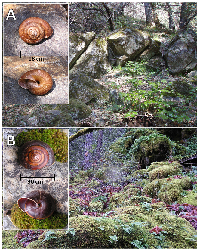
Populations of M. churchi are described as inhabiting many of same forest cover-type conditions described for M. setosa, but they are generally linked with open stands and exposed slopes, limestone outcrops, caves, talus slides, lava rockslides, and riparian corridors with deciduous understory associated with nearby forest debris in heavy shade (Fig. 2A; Roth 1981). Many sites around Shasta Lake consist of remnant shrub associations, various species of buck brush (Ceanothus sp.), manzanita (Arctostaphylos manzanita), and pine-oak woodland (Hanna and Smith 1933). Conversely, populations of M. setosa are typically found within mesic montane and mixed conifer-hardwood forests and riparian corridors, and occasionally upland environs dominated by sclerophyllous deciduous hardwood understories (Fig. 2B; Sullivan 2021a, b).

Survey Methods and Data Collection

I derived predictor variables to assess geographic variation in co-occurring samples of M. setosa and M. churchi using Landsat Visual Ecological Groupings of vegetation-types (i.e., CALVEG; USFS 1981) and California Wildlife Habitat Relationships (CWHR; Airola 1988; Mayer and Laudenslayer 1988; Goodchild et al. 1991; Sawyer and Keeler-Wolfe 1995; Garrison et al. 2002). GIS-based CWHR layers provided information on forest stand structure at a ~16.2-ha minimum mapping unit; and a minimum mapping size of ~2.5-ha pixels was used to contrast environmental variables associated with each sample site. I used 18 environmental predictor variables including a seasonal component of environmental variance (mean monthly minimum and maximum temperature and mean monthly precipitation; Table 1) to evaluate macroscale habitat relationships between species. From these variables I created four sets of covariate categories: 1) Forest Cover Type [CWHR]; 2) Forest Stand Structure [i.e., CALVEG]; 3) Mesoscale Climate (geo-rectified raster data, PRISM Climate Group [2023]; Daly et al. 2008); and 4) Exposure-Distance to Nearest Stream (henceforth referred to as Exposure-Distance), to describe attributes of the landscape (scale = 10-m digital elevation models). I used Inverse Distance Weighting (IDW; GISGeography 2023) to produce deterministic multivariate geographic interpolation maps from a scattered set of points depicting variance in summer and winter precipitation and temperature across the co-occupied species landscape (QGIS Development Team 2021).

Table 1. Categories and individual biotic and abiotic environmental variables, classification codes, and plant species assemblages used to compare macroscale variance between samples of co-occurring samples of M. churchi and M. setosa.

Predictor variable	Description
1. Cover-type	CWHR Forest Stand Vegetation Cover-Types: AGS = Annual grassland, BAR = Barren, BOP = Blue oak-foothill pine, CPC = Closed-cone pine cypress, DFR = Douglas fir, JPN = Jeffrey Pine, Ponderosa Pine, Sugar Pine, KMC = Klamath mixed conifer, MCH = Mixed chaparral, MCP = Montane chaparral, MHC = Montane hardwood conifer, MHW = Montane hardwood , PPN = Ponderosa pine, SCN = Subalpine conifer, SMC = Sierran mixed conifer, WFR = White fir.
2. Conifer Cover from above (CCFA) 3. Hardwood cover from above (HCFA) 4. Over-story Tree Diameter (OSTD) 5. Total Tree cover from above (TCFA) 6. Tree Size Class (TSIZ) 7. Soil-type (MUSYM)	Forest Stand Attributes: CALVEG vegetation cover from above (mapped vegetation [%] cover [crown] from above) as delineated by aerial photos. Total tree cover from above, conifer tree cover from above, and hardwood cover from above were mapped as a function of canopy closure in 10% cover classes: 0 (< 1%), 5 (1–9%), 15 (10–19%), 25 (20–29%), 35 (30–39%), 45 (40–49%), 55 (50–59%), 65 (60–69%), 75 (70–79%), 85 (80–89%), and 85 (90–100%). CALVEG overstory tree diameter class mapped over-story tree diameter class of mixed tree types using average diameter at breast height (DBH = 1.37 m above ground) for trees forming the uppermost canopy layer (Helms 1998) using average basal area (Quadratic Average Diameter or QMD; Curtis and Marshall 2000) of top tree story categories: 1 = seedlings (0–2.3 cm QMD), 2 = saplings (2.5–12.5 cm QMD), 3 = poles (12.7–25.2 cm QMD), 4 = medium sized trees (50.8–76.0 cm QMD), and 5 = large sized trees (> 76.2 cm QMD). Tree size classification derived from mapped attributes corresponding to parameters derived from the CALVEG and CWHR systems. Tree size codes (ranked): 1 = seedling tree, 2 = sapling tree, 3 = pole tree, 4 = small tree, 5 = medium-large tree, and 6 = multilayered tree. Specific soil-types were derived from USDA-NCSS soil survey data (SSURGO 2023) and verified regionally by use of the University of California U.C. Davis Soil Research Lab (UCD 2023).
8. Evapotranspiration (EVAP mm) 9. Summer Temperature (TASM ℃) 10. Winter Temperature (TAWN ℃) 11. Summer Precipitation (PASM mm) 12. Precipitation (PAWN mm) 13. Minimum Temperature (TMIN1-12 ℃) 14. Maximum Temperature (TMAX1-12 ℃) 15. Average Precipitation (PPT1-12 mm)	Average Monthly Mesoscale Climatic Attributes Climate attributes were derived from the PRISM (Parameter-elevation Regressions on Independent Slope Model; Daly et al. 1994; Daily et al. 2008), where long-term average datasets were modeled using a spatially gridded digital elevation model (DEM) as the predictor grid for specific climatological periods.
16. Aspect (ASPC) 17. Elevation (ELEV m) 18. Hill-shade (HLSD) 19. Slope (SLOP) 20. Distance to Nearest Stream (DNST m)	Exposure-Distance to Nearest Stream: Maps of aspect, elevation, hill-shade, and slope were all derived from a United States Geological Survey (USGS) Digital Elevation Model (DEM) based on a 1:250,000-scale/3-arc second data resampled to 10-m resolution. Aspect was obtained from a raster surface that identified down-slope direction of maximum rate of change in value from each cell to its neighbors. Equates to slope direction and values of each cell in the output raster show compass direction of surfaces measured clockwise in degrees from zero (due north) to 360° (Burrough and McDonell 1998). Degrees of aspect in relative in direction were north (0°), east (90°), south (180°), and west (270°). Values of cells in an aspect dataset indicate direction cell’s slope faces. Flat areas having no down slope direction were given a value of -1 in the model. Aspect was quantified by use of aspect degrees binned into one of eight 45° ordinal categories (N, NE, E, SE, etc.). Elevation (m) was obtained from vertical units of a spaced grid with values referenced horizontally to UTM projections referenced to North American Datum NAD 83. Hill-shade was obtained from a shaded relief raster (integer values ranging from 0–255) where the source of illumination was considered infinite. The output raster only considered local illumination angle. Analysis of shadows considered effects of local horizon at each cell. Shadowed raster cells received a value of zero. Slope was obtained from a raster surface that identified gradient or rate of maximum change in z-value from each cell of a raster surface. It relates maximum change in elevation over distance between a cell and its eight neighbors, thus identifying the steepest downhill descent from the cell (Burrough and McDonell 1998). Range of slope values (degrees): flat (0°), steep (35°–45°), moderate (5°–8.5°), to very steep (> 45°). Distance to the nearest stream was obtained from CDFW GIS Clearing house (CDFW 2023).

Statistical Analyses

I performed all statistical tests using R software (R Core Team 2023) and set statistical significance at α < 0.05. I evaluated the density distribution (i.e., histograms) of each habitat parameter to the expected theoretical density distributions (i.e., Normal vs. Gamma) using the Akaike’s goodness of fit criterion (AIC; Akaike 1973). Although results showed that the frequency distributions of most variables approximated a normal distribution for both species the remainder followed a Gamma distribution (Appendix I; Appendix II). Additionally, I evaluated univariate normality in macroscale habitat parameters using the adjusted Anderson-Darling test (AD; Razali and Wah 2011) in which all tests for normality failed (Table S1). Thus, I used nonparametric statistics to evaluate significance in all follow-on tests of environmental parameters for all group comparisons and a Gamma distribution was used for all regressions. I used the Wilcoxon signed rank (V) test with continuity correction to compare the relative percentages of forest-types between species and I used a modified Dunn Test (x², function “dunn.test”, altp = TRUE) to change the output to a two-sided P-value when comparing species with respect environmental attributes (Cross Validated 2023). All nonparametric P-values were adjusted using the Bonferroni correction method (a = 0.95) to counteract the problem of inflated Type I errors (Everitt and Hothorn 2011; Josse and Husson 2016).

I used Principal Components Analysis (PCA) modeled for missing data (Josse and Husson 2016) on scaled (i.e., standardized) variables to identify the extent of association among habitat attributes, and to assess the relative ability of each parameter to explain variation between species (Everitt and Hothorn 2011; Sullivan 2022a,b). I tested for significant differences in overall habitat “similarity” based on results of the first three components (i.e., PC I–PC III) between species using permutation-based multivariate analysis of variance (PERMANOVA; package “vegan” function “adonis2”, 1,000 permutations; Oksanen et al. 2013; R Core Team 2023) followed by individual pairwise comparisons of each component by use of the modified Dunn Test. PERMANOVA is a permutation-based technique that makes no distributional assumptions about multivariate normality or homogeneity of variances (Anderson 2017). Because it is based on a distance matrix, PERMANOVA can be applied identically to both univariate and multivariate data. Further, the test statistic is identical to the conventional F-statistic when calculated using Euclidean distance for a single variable (Vicente-Gonzalez and Vicente-Villardon 2021).

I used Generalized Additive Modeling (GAM) in all regressions and a Gamma error-structure to establish the relationship between response variables and the smoothed functions of predictor variables (Wood et al. 2016; Wood 2017). Statistics reported from each GAM included: 1) t-statistic (~significance of smooth lines in the regression) ; 2) Dev.Exp. (proportion of null deviance explained most appropriate for non-normal errors); and 3) P-value plus 95% confidence bands for spline lines (Nychka 1988). In all GAMs I set the base dimension at k = 3 degrees of freedom for each smooth line. Spearman’s rank correlation coefficient was used as a follow-on statistic to assess the strength and significance of trends in data delineated by smooth terms (Diankha and Thiaw 2016). I used the “gghdr” package to plot the highest density regions (HDR) of the underlying probability distribution (i.e., 50% to > 99% HDRs) in all regressions. Here, gghdr identified any multimodal relationship between a response and predictor variable in which a credible unobserved parameter interval falls within a particular probability distribution (Hyndman 1996). I performed multiple Spearman correlation analyses (r_s; 2-tailed test) among the quantitative and ordinal habitat variables to test for potential multicollinearity and evaluate the strength and direction of the relationship between pairs of variables whether linear or not (Corder and Foreman 2014).

Results

Species Intra- and Inter-specific Distances between Co-occurring Samples

My estimate of the potential extent of co-occurrence between M. churchi and M. setosa was ~1,256.6 km² in total area (perimeter = ~125.7 km) based on a minimum spanning polygon surrounding the hypothesized area of overlap (Fig. 1). As with the known range of both species, I view my estimate of co-occupancy to be conservative pending more extensive sampling in all cardinal directions. PCA of the extent of co-occurrence between species based on geographic coordinates and elevation (i.e., UTM-E, UTM-N, ELEV) showed that variable loadings (i.e., correlations) were high and positive for both UTM coordinates (i.e., 0.773, 0.85) but negative (i.e., -0.882) for elevation along PC I (eigenvalue percentages), which accounted for 72.8% of the total variation along this eigenvector (Fig. 3A). Topographically, the distribution of co-occurring samples followed primarily a north-west and secondarily a south-east geographic direction that included both sides of the mainstem Trinity and South Fork Trinity Rivers and the headwaters of the upper Mad River. This geographic orientation was clearly illustrated by the 95% confidence ellipses surrounding samples of each species in 2- dimensional space.

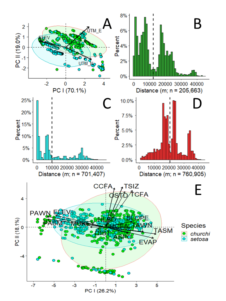
Based on UTM coordinates the average distance between samples based on GIS analyses was: 1) M. churchi: x̅ = 12.3 km (min = 0.0 km, max = 45.3 km), 2) M. setosa: x̅ = 9.9 km (min = 0.0 m, max = 45.7 km), and 3) M. churchi vs. M. setosa: x̅ = 20.7 km (min = 0.1 km, max = 48.2 km). Similarly, inter-specific minimum pair-wise distances derived from UTM coordinate between samples of M. churchi vs. M. setosa were considerably larger and much less frequently documented than between samples of only M. churchi or samples of only M. setosa. For example, there were 1,512 (n = 205,663; Fig. 3B) intra-specific pair-wise distances under 200 m for M. churchi and 88,546 (n = 701,407; Fig. 3C) for M. setosa, but only 16 (n = 760,905; Fig. 3D) inter-specific pair-wise distances under 200 m for co-occurring (i.e., parapatric) samples and no locations where both taxa had the same UTM coordinates.

Variance in Forest Cover- and Soil-types

In combined samples of both species, I identified a total of 15 CWHR landscape-level (i.e., macroscale) forest cover-types and 82 distinct soil-types. For M. churchi the most common forest-type was Sierra Mixed Conifer Forest (SMC = 39.9%) and Douglas Fir Forest (DFR = 28.9%; Fig. 4A). In M. setosa the forest-types were the same but with very different percentages (i.e., SMC = 78.8% and DFR = 14.8%). Not only did M. churchi occur at sites that were more diverse in forest vegetation, but these sites had also much higher minor percentages of Mixed chaparral (MHC = 7.1%), Montane Chaparral (MCP = 5.9%), Klamath mixed conifer (KMC = 4.9%), and White Fir (WFR = 4.2). Paired Spearman signed-rank correlations revealed a significant relationship in the relative proportions of various forest cover-types (r_s = 0.540, P = 0.039, n = 15) at sample sites between species. Similarly, results of paired Wilcoxon signed-rank tests showed a significant difference between taxa in the relative proportions of forest cover (V = 100, P = 0.020, n = 15).

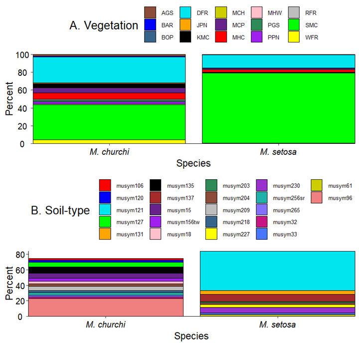
For soil-type I found 61 and 39 soil-type families associated with samples of M. churchi and M. setosa, respectively. Proportionally, stacked bar graphs of soil-type families accounting for > 2.0% of the total soil-types showed that samples of M. churchi consisted of a far greater diversity of soil-types than did samples of M. setosa (Fig. 4B), with musym96 (Hohmann-Neuns families complex, 40–60% slopes) being the most common (22.5%) soil-type among samples of M. churchi and musym121 (Holland, deep-Hugo families complex, 20–40% slopes) being the most dominant (50.6%) soil-type among samples of M. setosa (Table S2). Of these, the only soil-type shared by the two species was musym204 (Neuns family, 60 ̶ 80% slopes) at 3.1% for M. churchi and 2.1% for M. setosa. In soil-type the disparity between species was so great that it was not possible to test for a statistical difference. Further, there also were significant differences between species in all environmental attributes measured at each site and in monthly temperature and precipitation values, which reflected variance in the climatic regime on a season basis (Table 2; Appendix III; Appendix IV).

Table 2. Non-parametric Dunn’s Tests (P-values adjusted using Bonferroni correction) between co-occurring M. churchi and M. setosa for all environmental variables except monthly temperature and precipitation. Forest Stand Structure (CCFA = Conifer Cover from Above, HCFA = Hardwood Cover from Above, OSTD = Over-story Tree Diameter, TCFA = Total Tree Cover from Above, TSIZ = Tree Size Class, MUSYM = Soil Type); Mesoscale Climate (EVAP = Evapotranspiration, PASM = Average Annual Summer Precipitation, PAWN = Average Annual Winter Precipitation, TASM = Average Annual Summer Temperature, TAWN = Average Annual Winter Temperature; Exposure-Distance (ASPC = Aspect, DNST = Distance to Nearest Stream (m), ELEV = Elevation, HLSD = Hill-shade, SLOPE = Slope. Average Monthly: Minimum and Maximum Temperature (TMIN, TMAN) and Precipitation (PPT).

Variable Category	Variable	ꭓ2	P-valuea
Forest Stand Structure	CCFA	8.0	<0.001***
Forest Stand Structure	HCFA	9.5	<0.001***
Forest Stand Structure	OSTD	1.1	0.268
Forest Stand Structure	TCFA	0.8	0.408
Forest Stand Structure	TSIZ	6.3	<0.001***
Forest Stand Structure	MUSYM	22.8	<0.001***
Mesoscale Climate	EVAP	15.9	<0.001***
Mesoscale Climate	PASM	5.9	<0.001***
Mesoscale Climate	PAWN	22.3	<0.001***
Mesoscale Climate	TASM	7.1	<0.001***
Mesoscale Climate	TAWN	12.7	<0.001***
Exposure-Distance	ASPC	10.2	<0.001***
Exposure-Distance	DIST	12.5	<0.001***
Exposure-Distance	ELEV	13.1	<0.001***
Exposure-Distance	HLSD	5.6	<0.001***
Exposure-Distance	SLOPE	2.5	<0.013**
x̅ Monthly Minimum Temperature	TMIN1	22.0	<0.001***
x̅ Monthly Minimum Temperature	TMIN2	19.1	<0.001***
x̅ Monthly Minimum Temperature	TMIN3	16.9	<0.001***
x̅ Monthly Minimum Temperature	TMIN4	16.4	<0.001***
x̅ Monthly Minimum Temperature	TMIN5	17.3	<0.001***
x̅ Monthly Minimum Temperature	TMIN6	14.8	<0.001***
x̅ Monthly Minimum Temperature	TMIN7	8.0	<0.001***
x̅ Monthly Minimum Temperature	TMIN8	8.1	<0.001***
x̅ Monthly Minimum Temperature	TMIN9	7.5	<0.001***
x̅ Monthly Minimum Temperature	TMIN10	10.2	<0.001***
x̅ Monthly Minimum Temperature	TMIN11	21.8	<0.001***
x̅ Monthly Minimum Temperature	TMIN12	21.9	<0.001***
x̅ Monthly Maximum Temperature	TMAX1	11.4	<0.001***
x̅ Monthly Maximum Temperature	TMAX2	4.1	<0.001***
x̅ Monthly Maximum Temperature	TMAX3	3.0	<0.010**
x̅ Monthly Maximum Temperature	TMAX4	3.5	<0.001***
x̅ Monthly Maximum Temperature	TMAX5	3.2	<0.001***
x̅ Monthly Maximum Temperature	TMAX6	3.5	<0.001***
x̅ Monthly Maximum Temperature	TMAX7	3.4	<0.001***
x̅ Monthly Maximum Temperature	TMAX8	3.4	<0.001***
x̅ Monthly Maximum Temperature	TMAX9	2.8	<0.002**
x̅ Monthly Maximum Temperature	TMAX10	3.1	<0.001***
x̅ Monthly Maximum Temperature	TMAX11	3.1	<0.001***
x̅ Monthly Maximum Temperature	TMAX12	4.0	<0.001***
x̅ Monthly Precipitation	PPT1	13.7	<0.001***
x̅ Monthly Precipitation	PPT2	14.3	<0.001***
x̅ Monthly Precipitation	PPT3	15.0	<0.001***
x̅ Monthly Precipitation	PPT4	16.5	<0.001***
x̅ Monthly Precipitation	PPT5	14.3	<0.001***
x̅ Monthly Precipitation	PPT6	14.0	<0.001***
x̅ Monthly Precipitation	PPT7	16.8	<0.001***
x̅ Monthly Precipitation	PPT8	13.5	<0.001***
x̅ Monthly Precipitation	PPT9	17.6	<0.001***
x̅ Monthly Precipitation	PPT10	16.7	<0.001***
x̅ Monthly Precipitation	PPT11	16.3	<0.001***
x̅ Monthly Precipitation	PPT12	16.8	<0.001***

Environmental Attributes between Species

PCA of all environmental parameters accounted for 57.8% of the dispersion (variance) contained in the data on the first 3-eigenvectors (Table 3). Vector loadings, direction, and the relationship of each attribute arrow showed that monthly Average Evapotranspiration and Summer and Winter Temperatures had the highest positive loadings along PC I (26.2%; Fig. 3E). This contrasted sharply with Average Summer and Winter Precipitation, and Elevation, which loaded negatively along PC I. All attributes associated with forest stand structure loaded heavily along PC II (18.1%) except Hardwood Overstory Cover, which was largely typical of M. churchi landscapes. Scatter plots of the two PC scores showed the extent of overlap in ecological niche space between the two species. PERMANOVA of factor loadings of individuals showed a significant global difference between species based on the first three components (F = 213, df = 1, 1291, P < 0.001) and post-hoc Dunn’s multiple rank sums test showed that each species differed significantly along vectors of multivariate macroscale habitat (PC 1: χ² = 7.7, P < 0.001; PC 2: χ²= 5.1; P < 0.001; PC III: χ²= 17.3, P < 0.001). IDW interpolation maps of geographic variance in seasonal mesoclimate showed that samples of M. churchi primarily fell within dryer and slightly cooler topography. Whereas samples of M. setosa fell within wetter and slightly warmer areas within co-occupied topography (Fig. 5A–D) within warmer low elevation more humid riparian tributaries to major river systems throughout the basin (Table S1).

Table 3. Principal components analysis (PCA) of macroscale environmental parameters on the first three dimensions. (PC = Principal Component)

Table 3a. Eigenvalues for each principal component.

Eigenvalues	PC I	PC II	PC III
Variance	4.2	2.9	2.2
Explained (%)	26.2	18.1	13.6
Cumulative (%)	26.2	44.2	57.8

Table 3b. Forest Stand Structure variable correlations with components. (CCFA = Conifer Cover from Above, HCFA = Hardwood Cover from Above, OSTD = Over-story Tree Diameter, TCFA = Total Tree Cover from Above, TSIZ = Tree Size Class, MUSYM = Soil-type)

Variable	PC I	PC II	PC III
CCFA	0.129	0.837	–0.314
HCFA	0.364	–0.017	0.527
OSTD	0.286	0.761	0.107
TCFA	0.396	0.783	0.096
TSIZ	0.250	0.856	0.178
MUSYM	–0.225	0.007	0.253

Table 3c. Mesoscale Climate variable correlations with components. (EVAP = Evapotranspiration, PASM = Average Annual Summer Precipitation, PAWN = Average Annual Winter Precipitation, TASM = Average Annual Summer Temperature, TAWN = Average Annual Winter Temperature)

Variable	PC I	PC II	PC III
EVAP	0.709	-0.232	0.375
PASM	–0.859	0.170	0.278
PAWN	–0.864	0.226	–0.206
TASM	0.747	–0.145	–0.551
TAWN	0.558	–0.097	–0.736

Table 3d. Exposure-Distance variable correlations with components (ASPC = Aspect, DNST = Distance to Nearest Stream (m), ELEV = Elevation, HLSD = Hill-shade, SLOPE = Slope.

Variable	PC I	PC II	PC III
ASPC	0.334	–0.123	0.540
DNST	–0.123	–0.041	0.283
ELEV	–0.741	0.252	–0.262
HLSD	0.015	0.062	0.322
SLOPE	0.395	0.123	0.165

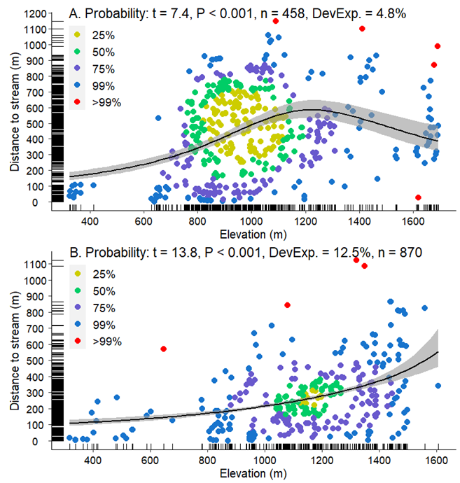
Relationship between Elevation and Distance to Nearest Stream

In the area of co-occurrence, the two species differed significantly in Distance to Nearest Stream (χ² = 12.2, df = 1, P < 0.001) and Elevation (χ² = 13.2, df = 1, P < 0.001).Average Distance to Nearest Stream for M. churchi was 441.1 m (min = 1.1 m, max = 1,147.0 m) and average Elevation was 999.9 m (min = 325.0 m, max = 1,692 m). When compared to samples of M. setosa Distance to the Nearest Stream averaged 269.4 m (min = 0.4 m, max = 1,122.2 m) and Elevation averaged 1,136.6 m (318.0 m, max = 1,605.0 m). In both situations Distance to Nearest Stream was substantially smaller and Elevation higher in mesic populations of M. setosa than it in samples of M. churchi. Although GAM regression of Distance to Nearest Stream vs. Elevation was positive and significant for both taxa (Fig. 6A,B), correlations between response and predictor variables were not strong in either species (M. churchi: r_s = 0.250, P < 0.001 and M. setosa: r_s = 0.380, P < 0.001). Nonetheless, the relationship between Distance to Nearest Stream and Elevation in both species was considerably stronger than between Distance to Nearest Stream and any other macroscale attribute (Tables S3, S4). Examination of HDR’s in each GAM showed that in M. churchi samples consisted of a large HDR centered at ~500 m from the nearest stream (y-axis) and ~900 m in elevation (x-axis; Fig. 6A). For M. setosa the HDR cluster was much smaller ~1,180 m in Elevation and 200 m from the nearest water source (Fig. 6B).

Discussion

Pair-wise Distance and Co-occurrence

In widely distributed taxa there may, on occasion, be areas where two or more closely related species co-occur. Therefore, it is important to define what kind of co-occurrence between species this spatial relationship may entail. My study was designed to determine the spatial extent of habitat co-occupancy and importance of macroscale ecological variance in the overlapping geographic distribution of M. churchi and M. setosa. Analysis of inter-species pair-wise distances based on UTM coordinates showed that there was no overlap in the sample of data I used, which signals that the two species are not syntopic, or parapatric, but “microsympatric.” The finding that Elevation in samples of M. setosa was on average higher than in samples of M. churchi also indicates lack of syntopy between taxa in relative proximity. Invoking microsympatry between species therefore necessitates quantification of inter-species spacing within the area of co-occurrence, which in each instance will be unique to each pair of species.

Mumladze (2014) concluded that the distinctness of ecological niches at a larger scale (i.e., macrohabitat) than microhabitat patches was not the primary factor in shaping the local spatial pattern of two species of helicoid snails (genus Helix) and that other factors (e.g., competition, predation, anthropogenic disturbance, etc.) likely played a more significant role in limiting the local spatial pattern and ecological tolerance of both species. However, I found that ecological variance in co-occurring samples of M. churchi and M. setosa showed significant differences in macroscale categories of forest-, vegetation-, and soil-type diversity (particularly in M. churchi), and continuously distributed environmental variables. Significant differences in mesoscale monthly (i.e., seasonal) precipitation and temperature between species also likely reflect threshold tolerances in regional parameters regulated by variance in thermal and moisture regimes at a landscape level. Similarly, other studies (Gheoca et al. 2021) also suggest that habitat continuity, an arguably macroscale parameter, was the main factor affecting snail abundance and species richness of communities of terrestrial gastropods in riparian forests. As relates to soil-type, no assessments were made at the time surveys were conducted that would allow any detailed understanding of the chemical composition of the soil type(s) associated with each taxon, which would require a microhabitat assessment to determine the nature and significance from a functional physiological perspective.

Thus, in the present example a more detailed proximate-level (i.e., microscale) habitat assessment of the few areas of relative proximity and additional surveys may reveal sites with a heterogenous environment allowing co-occurrence of these two taxa. Future habitat studies in these areas seem warranted because failing to discover M. churchi at a site where M. setosa is present is only circumstantial evidence that M. churchi does not occur there, even though these species have, to date, never been found in syntopy (Roth and Pressley 1986). Inclusive of microsympatric associations with M. setosa, M. churchi continues its historical biogeographic legacy of inhabiting drier and warmer habitats throughout its geographic distribution as reflected in mean annual temperature and precipitation and seasonal variance in these metrics. Moreover, viability in populations of M. setosa continues to be tied to availability of mesic habitat of dense understory shading, temperature- and humidity-regulating conifer and riparian woodlands and scattered stable saxicolous habitat that collectively facilitate long-term survival and reproduction (Roth 1978, 1981; Sullivan 2022b).

Conclusions and Recommendations

Here, I assessed the extent of proximity and similarity in macroscale environmental attributes of M. churchi and M. setosa. Future inventories in areas of potential co-occurrence previously not surveyed for both species combined with more proximate finer-scale analyses of site-specific microhabitat, above and below ground, focused on thermal and moisture regimes will be required to understanding habitat differences for these species (Sullivan 2022b). Identifying critical environmental factors associated with foraging habitat can also help explain inter-species habitat preferences and provide a baseline for detecting shifts in species distributions based on fluctuating temperature and precipitation regimes effected by regional climate change in future decades. Therefore, understanding the mechanisms by which taxonomically similar species of terrestrial snails co-occur would seem to require: 1) quantification of inter-species spacing at both a macro- and micro-scale, and a detailed exploration of their 2) fundamental niches (i.e., resources and conditions that they could use), 3) realized niches (i.e., resources and conditions that they are using), and 4) behavioral responses to other taxa when in close proximity (Soberón 2007).

Acknowledgments

I thank all anonymous reviewers for their helpful editorial comments. I am particularly grateful for the financial support and assistance provided by the U.S. Fish and Wildlife Service (Project T-21-1 [Project C]) through the State Wildlife Grant (SWG) Program.

Literature Cited

• Airola, D. A. 1988. A guide to the California wildlife habitat relationships system. California Department of Fish and Game, Sacramento, CA, USA.
• Akaike, H. 1973. Information theory and an extension of the maximum likelihood principle. Pages 267–281 in B. N. Petrov and F. Csáki, editors. 2nd International Symposium on Information Theory, Tsahkadsor, Armenia, Budapest, USSR.
• Anderson, M. J. 2017. Permutational multivariate analysis of variance (PERMANOVA). In Wiley StatsRef: Statistics Reference Online. N. Balakrishnan, T. Colton, B. Everitt, W. Piegorsch, F. Ruggeri, and J. L. Teugels, editors. https://doi.org/10.1002/9781118445112.stat07841
• Anderson, S., and M. K. Evensen. 1978. Randomness in allopatric speciation. Systematic Zoology 27:421–430.
• Bull, C. M. 1991. Ecology of parapatric distributions. Annual Review of Ecology and Systematics 22:19–36.
• Burrough, P. A., and R. A. McDonnell. 1998. Principles of Geographical Information Systems. Oxford University Press, Oxford, UK.
• California Department of Fish and Wildlife (CDFW). 2023. CDFW GIS Clearinghouse – program-specific data. Available from: https://wildlife.ca.gov/Data/GIS/Clearinghouse (Accessed: 16 October 2023).
• Corder, G. W., and D. I. Foreman. 2014. Nonparametric Statistics: A Step-by-Step Approach, John Wiley and Sons, Inc., Hoboken, NJ, USA.
• Cross Validated. 2023. Is dunn.test for two samples equivalent to wilcox.test? Stack Exchange. Available from: https://stats.stackexchange.com/questions/355990/is-dunn-test-for-two-samples-equivalent-to-wilcox-test (Accessed: 16 October 2023).
• Curtis, R. O., and D. D. Marshall. 2000. Why quadratic mean diameter? Western Journal of Applied Forestry 15(3):137–139.
• Daly, C., R. P. Neilson, and D. J. Phillips. 1994. A statistical-topographic model for mapping climatological precipitation over mountainous terrain. Journal of Applied Meteorology 33:140–158.
• Daly C., M. Halbleib, J. I. Smith, W. P. Gibson, K. Matthew, M. K. Doggett, G. H. Taylor, J. Curtis, and P. P. Pasteris. 2008. Physiographically-sensitive mapping of temperature and precipitation across the conterminous United States. International Journal of Climatology 28:2031–2064.
• Diankha, O., and M. Thiaw. 2016. Studying the ten years variability of Octopus vulgaris in Senegalese waters using generalized additive model (GAM). International Journal of Fisheries and Aquatic Studies 2016:61–67.
• Everitt, B. S., and T. Hothorn. 2011. An Introduction to Applied Multivariate Analysis with R. Springer, New York, NY, USA.
• Garrison, B. A., M. D. Parisi, K. W. Hunting, T. A. Giles, J. T. McNerney, R. G. Burg, K. J. Sernka, and S. L. Hooper. 2002. Training manual for California Wildlife Habitat Relationships System CWHR database version 8.0. 9th edition. California Wildlife Habitat Relationships Program, California Department of Fish and Wildlife, Sacramento, CA, USA.
• Gheoca V., A. M. Benedek, and E. Schneider. 2021. Exploring land snails’ response to habitat characteristics and their potential as bioindicators of riparian forest quality. Ecological Indicators 132:1–9.
• GISGeography. 2023. Inverse distance weighting (IDW) interpolation. Available from: https://gisgeography.com/inverse-distance-weighting-idw-interpolation/
• Goodchild, M., F. W. Davis, M. Painho, and D. M. Storns. 1991. The use of vegetation maps and geographic information systems for assessing conifer lands in California. Technical Report 91-23, National Center for Geographic Information and Analysis, University of California, Santa Barbara, CA, USA.
• Hanna, G. D., and A. G. Smith. 1933. Two new species of Monadenia from northern California. Nautilus 46:79–86.
• Heart, K. M., A. R. Iverson, I. Fujisaki, M. M. Lamont, D. Bucklin, and D. J. Shaver. 2018. Sympatry or syntopy? Investigating drivers of distribution and co‐occurrence for two imperiled sea turtle species in Gulf of Mexico neritic waters. Evolutionary Ecology 8(24):12656–12669.
• Hyndman, R. T. 1996. Computing and graphing highest density regions. The American Statistician 50:120–126.
• Jorgensen, S. E., and B. Fath. 2008. Encyclopedia of Ecology. Elsevier, Oxford, UK.
• Josse, J., and F. Husson. 2016. missMDA: a package for handling missing values in multivariate data analysis. Journal of Statistical Software 70(1):1–31.
• King, M. 1993. Species Evolution: The Role of Chromosome Change. Cambridge University Press, Cambridge, MA, USA.
• Mayer K. E, and W. F. Laudenslayer. 1988. A Guide to the Wildlife Habitats of California. California Department of Forestry and Fire Protection, Sacramento, CA, USA.
• Mumladze, L. 2014. Sympatry without co-occurrence: exploring the pattern of distribution of two Helix species in Georgia using an ecological niche modelling approach. Journal of Molluscan Studies 80(3):249–255.
• Munz, P., and D. D. Keck. 1959. A California Flora. University of California Press, Berkeley, CA, USA.
• Nychka, D. 1988. Bayesian confidence intervals for smoothing splines. Journal of the American Statistical Association 83:1134–143.
• Oksanen, J., F. G. Blanchet, R. Kindt, P. Legendre, P. R. Minchin, R. B. O’Hara, and H. Wagner. 2013. Vegan: Community Ecology Package. R package version 2.0-10. Available from: https://cran.r-project.org/package=vegan
• Prism Climate Group. 2023. Northwest Alliance for Computational Science and Engineering. Oregon State University, Corvallis, OR, USA.
• Razali, N., and Y. B. Wah. 2011. Power comparisons of Shapiro-Wilk Kolmogorov-Smirnov, Lilliefors, and Anderson-Darling tests. Journal of Statistical Modeling and Analytics 2:21–33.
• Roth, B. 1978. Biology and distribution of Monadenia setosa Talmadge. Report to U.S. Forest Service, Shasta-Trinity National Forest, Redding, CA, USA.
• Roth, B. 1981. Shell color and banding variation in two coastal colonies of Monadenia fidelis (Gray) (Gastropoda: Pulmonata). Wasmann Journal of Biology 38:39–51.
• Roth, B., and L. L. Eng. 1980. Distribution, ecology, and reproductive anatomy of a rare land snail. Monadenia setosa, Talmage. California Fish and Game 66:4–16.
• Roth, B., and P. H. Pressley. 1986. Observations on the range and natural history of Monadenia setosa (Gastropoda: Pulmonate) in the Klamath Mountains, California, and the taxonomy of some related species. The Veliger 29:169–182.
• Roth, B., and P. S. Sadeghian. 2006. Checklist of the land snails and slugs of California. 2nd edition. Contributions in Science Number 3. Santa Barbara Museum of Natural History, Santa Barbara, CA, USA.
• Sawyer, J. O., and T. Keeler-Wolfe. 1995. A Manual of California Vegetation. California Native Plant Society, Sacramento, CA, USA.
• Soberón, J. 2007. Grinnellian and Eltonian niches and geographic distributions of species. Ecology Letters 10:1115–1123.
• Soil survey geographic database (SSURGO). 2023. Soil Survey Staff, Natural Resources Conservation Service, United States Department of Agriculture. Web Soil Survey. Available from: https://www.nrcs.usda.gov/resources/data-and-reports/soil-survey-geographic-database-ssurgo (Accessed: 16 October 2023).
• Sullivan, R. M. 2021. Phylogenetic relationships among subclades within the Trinity bristle snail species complex, riverine barriers, and re-classification. California Fish and Wildlife Journal, CESA Special Issue:107–145.
• Sullivan, R. M. 2022a. Macrohabitat suitability models for the Trinity bristle snail (Monadenia setosa) in the Greater Trinity Basin of northern California. California Fish and Wildlife Journal 108:e2.
• Sullivan, R. M. 2022b. Microhabitat characteristics and management of the Trinity bristle snail in the Greater Trinity Basin of northern California. California Fish and Wildlife Journal 108:e3.
• Sullivan, R. M. 2022c. Macroscale effects of the Monument Fire on suitable habitat of the Trinity bristle snail in the Greater Trinity Basin, Klamath Bioregion, northern California. California Fish and Wildlife Journal 108:e22.
• United States Department of the Interior (USFS). 1981. CALVEG: A Classification of California Vegetation. Pacific Southwest Region, Regional Ecology Group, San Francisco, CA, USA.
• University of California, Davis Soil Resource Lab (UCD). 2023. SoilWeb Apps. Available from: https://casoilresource.lawr.ucdavis.edu/soilweb-apps (Accessed: 16 October 2023).
• Vicente-Gonzalez, L., and J. L. Vicente-Villardon. 2021. PERMANOVA: Multivariate Analysis of Variance Based on Distances and Permutations. R Package, v.0.2.0. Available from: https://cran.r-project.org/package=PERMANOVA
• Welsh, H. H. 1994. Bioregions: an ecological and evolutionary perspective and a proposal for California. California Fish and Game 80:97–124.
• Wood, S. N. 2017. Generalized Additive Models: An Introduction with R. Chapman and Hall/CRC Press, Boca Raton, FL, USA.
• Wood, S. N., N. Pya, and B. Saefken. 2016. Smoothing parameter and model selection for general smooth models. Journal of the American Statistical Association 111:1548–1575.