---

The findings and conclusions in this article are those of the author and do not necessarily represent the views of the U.S. Fish and Wildlife Service. This paper was prepared under the auspices of the U.S. Government and is therefore not subject to copywrite.

REVIEW PAPER

Mark Gard*

California Department of Fish and Wildlife, Conservation Engineering Branch, 1010 Riverside Parkway, West Sacramento, CA 95605, USA  https://orcid.org/0009-0002-4529-9707

*Corresponding Author: mark.gard@wildlife.ca.gov

Published 21 Nov 2023 • doi.org/10.51492/cfwj.109.12

Abstract

Habitat suitability criteria (HSC) are a key information source used in designing habitat restoration projects. Many site-specific HSC have been developed in the Central Valley of California for various life stages of anadromous salmonids. Substantial differences between the HSC can be due to watershed characteristics and the methods used to develop the HSC. Spawning HSC generally have optimum depths of 0.3–1 m, optimum velocities of 0.3–1 m/s, and substrate sizes ranging from 25–100 mm. Optimum conditions for fry are generally shallow (less than 0.5 m) and slow (less than 0.1 m/s) with woody cover. Juvenile salmonids use deeper (0.5–1 m) and faster (up to 0.4 m/s) conditions than fry but are similar to fry in their preference for woody cover. HSC developed by the U.S. Fish and Wildlife Service on the Yuba River are recommended for evaluating habitat restoration projects on larger rivers, while HSC developed on Clear Creek are recommended for evaluating habitat restoration projects on smaller Central Valley streams. A key limitation of existing HSC is that they were only developed for in-channel conditions; fishery benefits of floodplain restoration projects are best quantified using total wetted area. Optimal HSC values are most useful in the initial design of habitat restoration projects, while flow-habitat relationships for existing versus proposed conditions can be useful in identifying needed design refinements, such as adding large woody debris.

Key words: Central Valley, Chinook Salmon, habitat suitability criteria, restoration, steelhead

Citation: Gard, M. 2023. Central Valley anadromous salmonid habitat suitability criteria. California Fish and Wildlife Journal 109:e12.

Editor: John Kelly, Fisheries Branch

Submitted: 11 April 2023; Accepted: 31 July 2023

Copyright: ©2023, Gard. This is an open access article and is considered public domain. Users have the right to read, download, copy, distribute, print, search, or link to the full texts of articles in this journal, crawl them for indexing, pass them as data to software, or use them for any other lawful purpose, provided the authors and the California Department of Fish and Wildlife are acknowledged.

Funding: The study was funded by the Anadromous Fisheries Restoration Program (Section 3406[b][1]) of the Central Valley Project Improvement Act (Title XXXIV of P.L. 102-575).

Competing Interests: The author has not declared any competing interests.

Introduction

Habitat suitability criteria (HSC) are used to translate physical parameters, such as depth and velocity, into habitat (Bovee et al. 1998). Additional uses of HSC are to predict niche requirements, species spatial distribution, deal with invasive species risk, species conservation (present distribution, restoration, etc.), and environmental impacts such as climate change, watershed development and pollution (Hirzel and Le Lay 2008). The focus of this paper is on the use of HSC to design habitat restoration projects for anadromous salmonids in the Central Valley of California, as well as to assess the success of habitat restoration projects through biological verification. Assessing predictive power of suitability criteria (and associated models) is of paramount importance, both theoretical and applied (Manly et al. 2002). HSC are used heavily in restoration design (Peterson and Duarte 2020), as well as planning for California infrastructure, water use in face of growing population, increased species listing, and a rapidly-changing environment.

The earliest HSC, such as Bovee (1978), were generalized criteria based largely on best professional judgement. More recent site-specific HSC can be divided into three major categories: 1) use, 2) use/availability ratios, and 3) presence/absence data (Ahmadi-Nedushan et al. 2006). In contrast, HSC used in recent hydropower relicensing are generally developed by consensus among the relicensing participants (for example, see South Sutter Water District 2018). Generally, separate HSC are developed for different life stages (spawning, fry rearing and juvenile rearing). Spawning HSC will usually include substrate, in addition to depth and velocity, while fry and juvenile rearing can include cover and adjacent velocity as additional parameters (USFWS 1985, 1994, 1997a, 1997b, 2003, 2005a, 2005b, 2006, 2010a, 2010b, 2011a, 2011b). The goal of HSC is to reflect organisms’ selection of preferred habitat conditions (Manly et al. 2002). For anadromous salmonids, preferred habitat conditions are assumed to translate into increased growth and survival . Habitat selection can be biased by limited availability of preferred habitat conditions; use/availability ratios were proposed to address this issue but can result in overcorrection of the effects of availability (Thomas and Bovee 1993). More recently, logistic regressions, using data collected at both location with (presence, occupied) and without (absence, unoccupied) organisms, have been used to address the effects of availability in developing HSC (Knapp and Preisler 1999; Parasiewicz 1999; Geist et al. 2000; Goodman et al. 2018; Guay et al. 2000; Pearce and Ferrier 2000; Filipe et al. 2002; Tiffan et al. 2002; McHugh and Budy 2004; Tirelli et al. 2009).

The purpose of this paper is to provide a synthesis and analysis of site-specific HSC for Chinook Salmon (Oncorhynchus tschawytscha) and steelhead (Oncorhynchus mykiss) in the Central Valley.

Methods

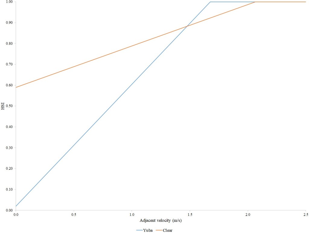
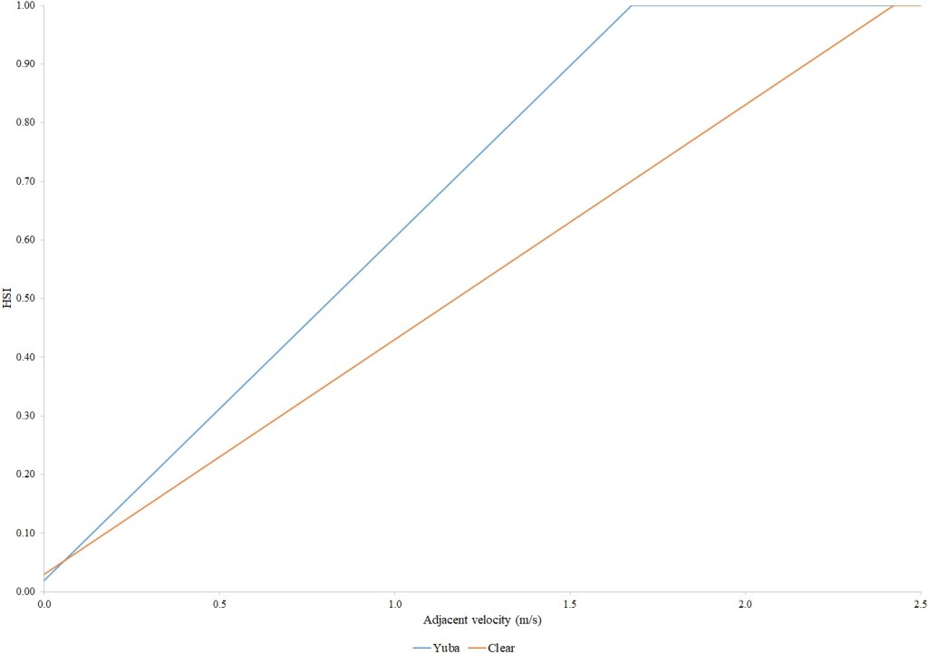
I reviewed gray literature (agency and consultant reports) to identify Central Valley anadromous salmonid site-specific HSC. Metadata for each set of HSC was assembled from either the gray literature or websites and Geographic Information System databases. Data for spawning HSC were generally collected by wading, with depth, mean water column velocity and substrate (Table 1) measurements collected at redd locations. For the Sacramento and Yuba Rivers, redds in deep (non-wadable) water were identified and their substrate quantified using underwater video, while the depth and velocity for each redd was measured using an Acoustic Doppler Current Profiler (ADCP; Gard and Ballard 2003). For presence/absence criteria, the horizontal location of redds within study sites were determined with either a total station or Real Time Kinematic Global Positioning System (RTK GPS) units; hydraulic models of the sites were then used to select unoccupied locations (USFWS 2005a, 2006, 2010a, 2011b). Data for fry and juvenile rearing HSC were collected by snorkeling, with numbered tags dropped at fish locations. Additional data recorded at fish locations were fish size, species, and cover code (Table 2). In general, there was an effort to sample equal areas of different mesohabitat types (riffles, runs, pools and glides) to address effects of availability on habitat use. Subsequently, measurements of depth, velocity, and adjacent velocity were made at each tag location. Adjacent velocity was defined as the fastest velocity within two feet laterally of a tag location. Adjacent velocity can be an important habitat variable as fish, particularly fry and juveniles, frequently reside in slow-water habitats adjacent to faster water where invertebrate drift is conveyed (Fausch and White 1981). For fry and juvenile rearing, the use of adjacent velocity is based on the mechanism of the transport of invertebrate drift from fast-water areas to adjacent slow-water areas where fry and juvenile salmonids reside via turbulent mixing. For the Sacramento and Yuba Rivers, rearing HSC data in deep (non-snorkelable) water was collected by SCUBA diving, with a weighted buoy placed at each fish location. Subsequently, depth and velocity data for each buoy, as well as at unoccupied locations, were measured with the ADCP. For presence/absence rearing criteria, depth, velocity, cover, and adjacent velocities were collected at randomly selected unoccupied locations (USFWS 2005b, 2010b, 2011a, 2013).

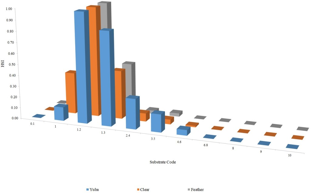
Table 1. Substrate codes, descriptors, and particle sizes (mm).

Code	Type	Particle Size
0.1	Sand/Silt	< 2.5
1	Small Gravel	2.5–25
1.2	Medium Gravel	25–50
1.3	Medium/Large Gravel	25–75
1.4	Gravel/Cobble	25–100
2.3	Large Gravel	50–75
2.4	Gravel/Cobble	50–100
3.4	Small Cobble	75–100
3.5	Small Cobble	75–125
4.5	Medium Cobble	100–125
4.6	Medium Cobble	100–150
6.8	Large Cobble	150–200
8	Large Cobble	200–250
9	Boulder/Bedrock	> 300
10	Large Cobble	250–300

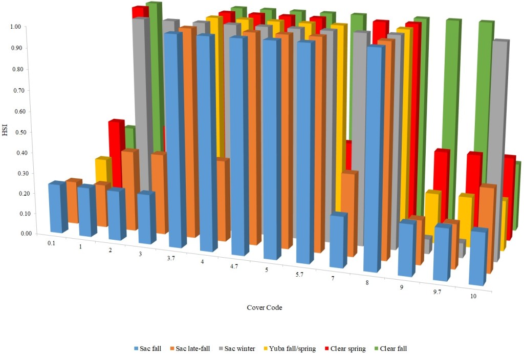
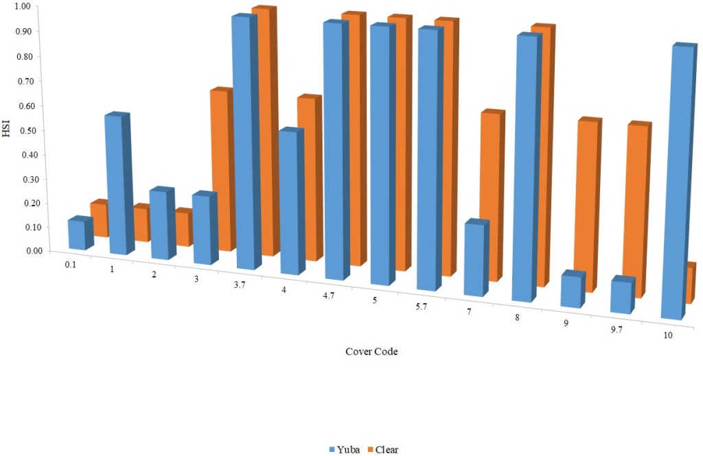
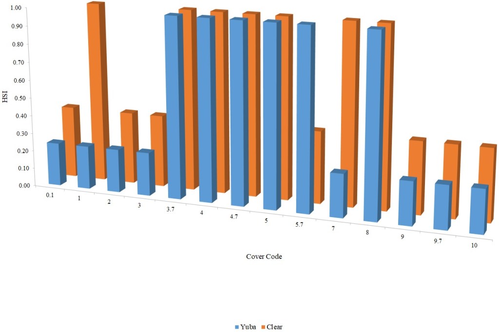
Table 2. Cover coding system.

Cover Category	Cover Code
No cover	0.1
Cobble (75–300 mm)	1
Boulder (> 300 mm)	2
Fine woody vegetation (< 25 mm diameter)	3
Fine woody vegetation + overhead	3.7
Branches	4
Branches + overhead	4.7
Log (> 300 mm diameter)	5
Log + overhead	5.7
Overhead cover (> 0.6 m above substrate)	7
Undercut bank	8
Aquatic vegetation	9
Aquatic vegetation + overhead	9.7
Rip-rap	10

For depth and velocity use HSC, the criteria were developed directly from use observations using a range of curve fitting and smoothing techniques. Use/availability criteria are developed by dividing use observations, generally binned, by availability data from transects. Presence/absence HSC are developed using a polynomial logistic regression that uses both the occupied and unoccupied data; the results of the logistic regression are rescaled, so that the highest value is 1.0, to calculate the Habitat Suitability Index (HSI) values. The first step in the development of the cover criteria was to group cover codes, so that there were no significant differences within the groups and a significant difference between the groups, using Pearson’s test for association. Categorical data (substrate and cover) are developed into HSC by calculating the frequencies for each substrate or cover code, and then dividing the frequencies by the highest frequency cover or substrate code, so that the highest HSI value is 1.0. For the Sacramento River, effects of availability on cover use were addressed by subsampling equal areas with and without woody cover (USFWS 2005b). This technique could not be used for the Yuba River and Clear Creek, due to the limited availability of woody cover. As a result, the HSI for each cover group was calculated by dividing the percent of occupied locations in each group by the percent of occupied locations in the group with the highest percent of occupied locations.

The resulting HSC, along with two-dimensional hydraulic and habitat models of study sites, were used to conduct biological verification. Specifically, one-tailed Mann-Whitney U tests (Zar 1984) were used to determine whether the combined suitability predicted by the hydraulic and habitat models was higher at locations where redds, fry, or juveniles were present versus locations where redds, fry, or juveniles were absent (USFWS 2005a, 2006, 2010a, 2010b, 2011b, 2013).

I conducted a meta-analysis of HSC by examining the correlation of optimal depths and velocities to watershed characteristics (flow and slope), and Kruskal-Wallis tests of the effects of HSC methods on optimal depths and velocities. Separate analyses were conducted for each life stage (spawning, fry rearing and juvenile rearing). I selected optimal depth and velocities as response variables because they are most commonly used in designing habitat restoration projects.

Results

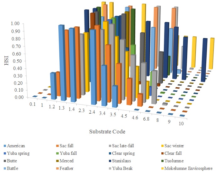
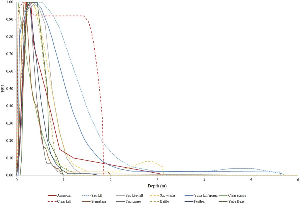
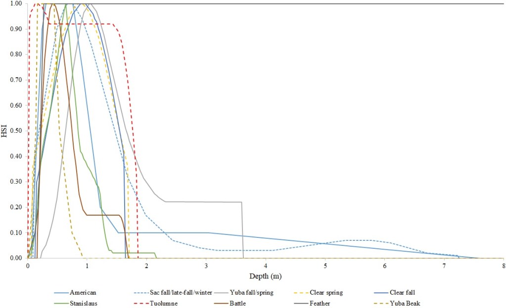
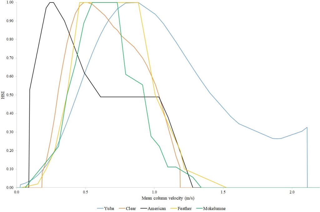
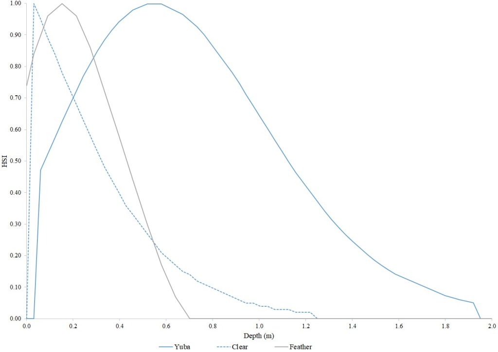
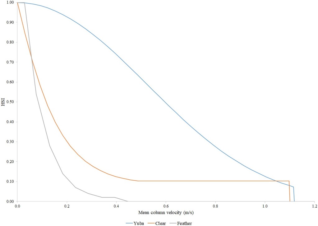
I identified seventeen sets of Central Valley site-specific HSC for Chinook Salmon spawning (Figs. 1–3), twelve sets of HSC for Chinook Salmon fry rearing (Figs. 4–7), ten sets of HSC for Chinook Salmon juvenile rearing (Figs. 8–11), five sets of HSC for steelhead spawning (Figs. 12–14), and three sets of HSC for steelhead fry and juvenile rearing (Figs. 15–22). References for the HSC are Aceituno (1990), Beak Consultants (1989), EBMUD (2019), Envirosphere (1991), Payne and Associates (1995, 2002), USFWS (1985, 1994, 1997a,b, 2003, 5005a,b, 2006, 2010a,b, 2011a,b, 2013), and Vogel (1982). For the Sacramento River, there were separate criteria for fall-run, late-fall-run and winter-run Chinook Salmon spawning and fry rearing, but only one set of criteria, for all three runs combined, for juvenile rearing. There were depth and velocity HSC for all sets of criteria, but not all spawning criteria had substrate HSC, and only half of the fry and rearing criteria had cover and adjacent velocity HSC. There were challenges in converting the substrate HSC used in different studies into a common substrate coding system, and the cover coding system in Table 2 limited the consideration of cover HSC to those that used this coding system. Other rearing HSC either did not use cover as a third parameter, used substrate, or used a simplified cover coding system with two categories (object present or absent). Metadata for the HSC (Table 3) showed a wide range of flows, gradients and techniques used to develop the criteria.

_

Table 3. Metadata for the Habitat Suitability Criteria that includes the river, species, run, life stage, number of observations, method used, flow (cfs), slope, months, and maximum fork length (max FL). (ND = No Data Available, NA = Not Applicable)

River	Species	Run	Life stage	# Obs	Method	Flow	Slope	Months	Max FL
American	Chinook	fall	spawning	218	Use	2,780	0.07%	Oct–Nov	NA
Sacramento	Chinook	fall	spawning	437	Use	5,237	0.10%	Oct–Nov	NA
Sacramento	Chinook	late-fall	spawning	156	Use	3,630	0.10%	Jan–Mar	NA
Sacramento	Chinook	winter	spawning	227	Use	13,843	0.10%	May–July	NA
Yuba	Chinook	spring	spawning	168	P/A	612	0.22%	Sept	NA
Yuba	Chinook	fall	spawning	870	P/A	681	0.22%	Oct–Nov	NA
Clear	Chinook	spring	spawning	180	P/A	167	0.44%	Sept–Oct	NA
Clear	Chinook	fall	spawning	761	P/A	217	0.44%	Oct–Dec	NA
Butte	Chinook	spring	spawning	792	P/A	99	0.72%	Sept–Oct	NA
Merced	Chinook	fall	spawning	186	Use	275	0.09%	Oct	NA
Stanislaus	Chinook	fall	spawning	105	U/A	400	0.11%	Nov	NA
Tuolumne	Chinook	fall	spawning	ND	Use	330	0.06%	ND	NA
Battle	Chinook	fall	spawning	216	Use	492	0.35%	Oct	NA
Feather	Chinook	fall	spawning	417	Use	1,550	0.03%	Oct–Dec	NA
Yuba	Chinook	fall	spawning	254	Use	737	0.22%	Nov	NA
Mokelumne	Chinook	fall	spawning	98	U/A	636	0.05%	fall	NA
Mokelumne	Chinook	fall	spawning	366	Use	323	0.05%	Oct–Jan	NA
American	Chinook	fall	fry	ND	Use	6,083	0.07%	ND	50
Sacramento	Chinook	fall	fry	407	P/A	8,133	0.10%	Jan–June	60
Sacramento	Chinook	late-fall	fry	439	P/A	9,902	0.10%	Apr–Sept	60
Sacramento	Chinook	winter	fry	266	P/A	9,356	0.10%	July–Jan	60
Yuba	Chinook	fall/spring	fry	178	P/A	1,859	0.22%	Jan–May	60
Clear	Chinook	spring	fry	201	P/A	241	0.44%	Nov–June	80
Clear	Chinook	fall	fry	316	P/A	224	0.44%	Jan–May	60
Stanislaus	Chinook	fall	fry	417	U/A	688	0.11%	Jan–April	49
Tuolumne	Chinook	fall	fry	ND	Use	300	0.06%	ND	ND
Battle	Chinook	fall	fry	353	Use	546	0.35%	ND	40
Feather	Chinook	fall	fry	369	Use	630	0.03%	Jan–May	50
Yuba	Chinook	fall	fry	180	Use	697	0.22%	ND	49
American	Chinook	fall	juvenile	ND	Use	3,700	0.07%	ND	100
Sacramento	Chinook	fall/late-fall/winter	juvenile	186	P/A	9,010	0.10%	Jan–Nov	ND
Yuba	Chinook	fall/spring	juvenile	39	P/A	1,411	0.22%	Mar–Sept	120
Clear	Chinook	spring	juvenile	191	P/A	221	0.44%	Nov–Sept	140
Clear	Chinook	fall	juvenile	170	P/A	140	0.44%	May-Sept	150
Stanislaus	Chinook	fall	juvenile	434	U/A	688	0.11%	Jan–Apr	150
Tuolumne	Chinook	fall	juvenile	ND	Use	540	0.06%	ND	ND
Battle	Chinook	fall	juvenile	155	Use	545	0.35%	Feb–May	80
Feather	Chinook	fall	juvenile	95	Use	630	0.03%	Jan–May	49
Yuba	Chinook	fall	juvenile	500	Use	381	0.22%	Apr–May	50
Yuba	steelhead	NA	spawning	184	P/A	2212	0.22%	Feb–Apr	NA
Clear	steelhead	NA	spawning	212	P/A	309	0.44%	Dec–July	NA
American	steelhead	NA	spawning	27	Use	1,660	0.07%	ND	NA
Feather	steelhead	NA	spawning	75	Use	600	0.03%	winter	NA
Mokelumne	steelhead	NA	spawning	152	Use	331	0.05%	Dec–Mar	NA
Yuba	steelhead	NA	fry	195	P/A	1,528	0.22%	May–Jan	60
Clear	steelhead	NA	fry	426	P/A	220	0.44%	Jan–Nov	80
Feather	steelhead	NA	fry	452	Use	630	0.03%	ND	50
Yuba	steelhead	NA	juvenile	74	P/A	1,316	0.22%	May–Dec	200
Clear	steelhead	NA	juvenile	191	P/A	221	0.44%	Nov–Sept	200
Feather	steelhead	NA	juvenile	527	Use	670	0.03%	ND	ND

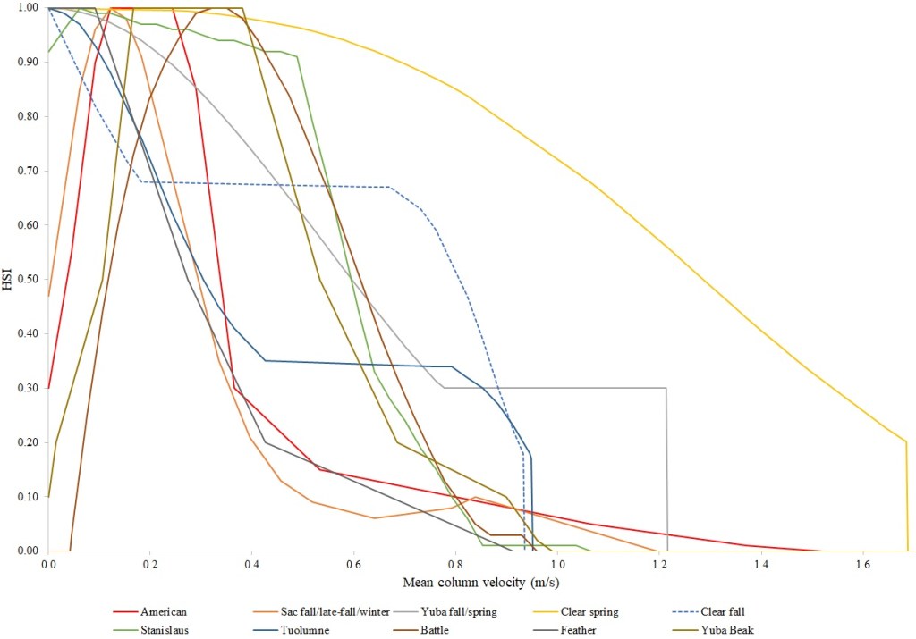
For Chinook Salmon spawning, all but one of the HSC sets had optimal depths in the range of 0.29–0.914 m. The outlier was Clear Creek spring-run Chinook Salmon, with an optimal depth of 1.829 m. The other large-scale pattern in the Chinook Salmon spawning HSC was the largest depth with a non-zero suitability; notably, three of the four HSC with the largest non-zero-suitability depth were from the Sacramento River. The other major factor affecting this pattern was the use of the Gard (1998) method to adjust depth suitability for availability, which was used on the five HSC with the largest non-zero-suitability depths. In contrast, velocities had a large degree of overlap between rivers, with optimal velocities ranging from 0.427–0.914 m/s. Substrate HSC were consistent showing optimal suitability for substrate codes 1.3 and 2.4. The Stanislaus and Mokelumne rivers HSC were outliers, however, showing relatively high suitability for large cobbles.

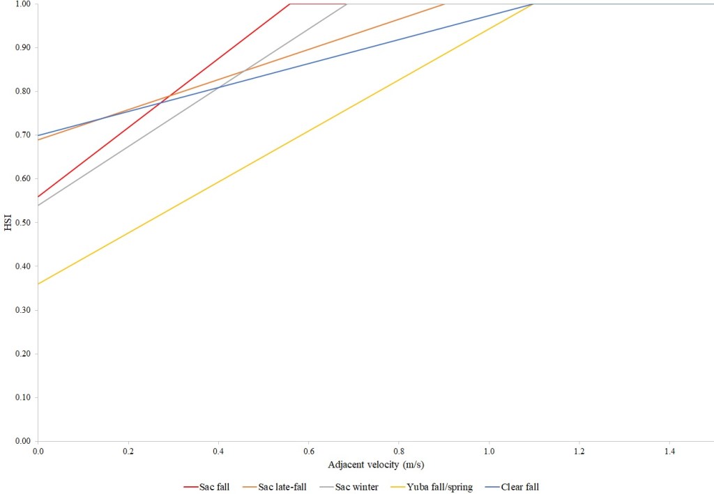
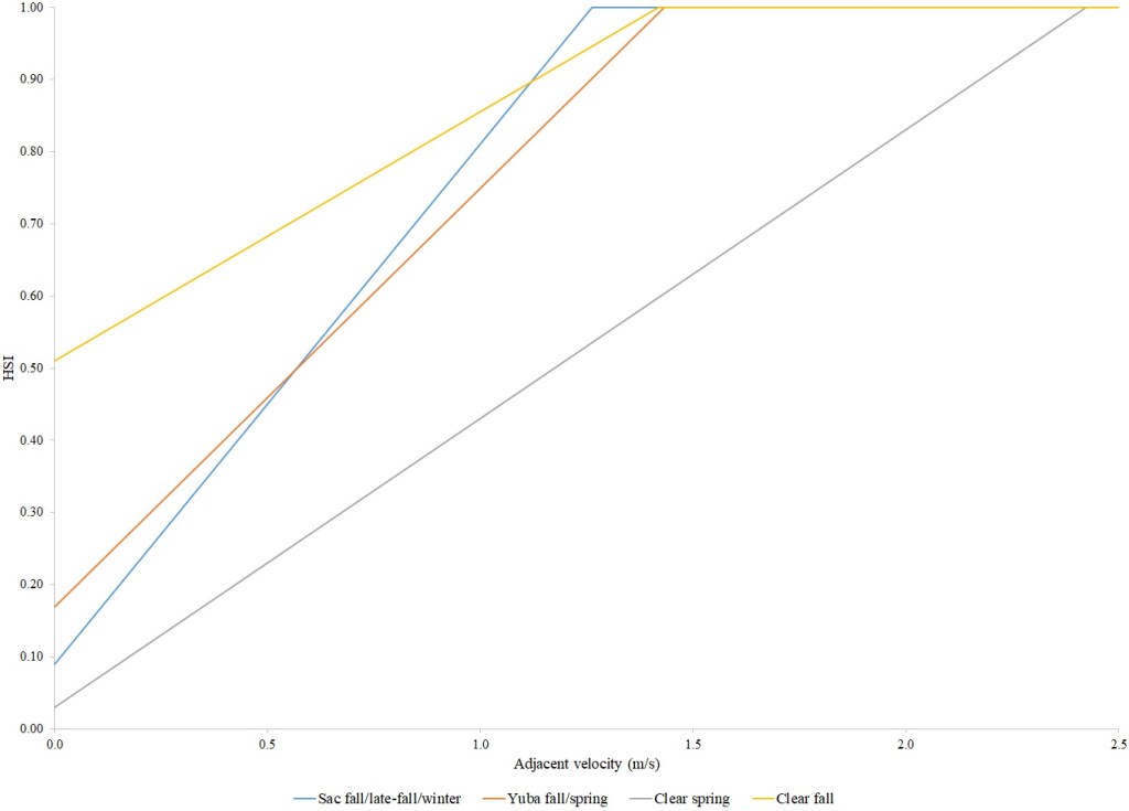
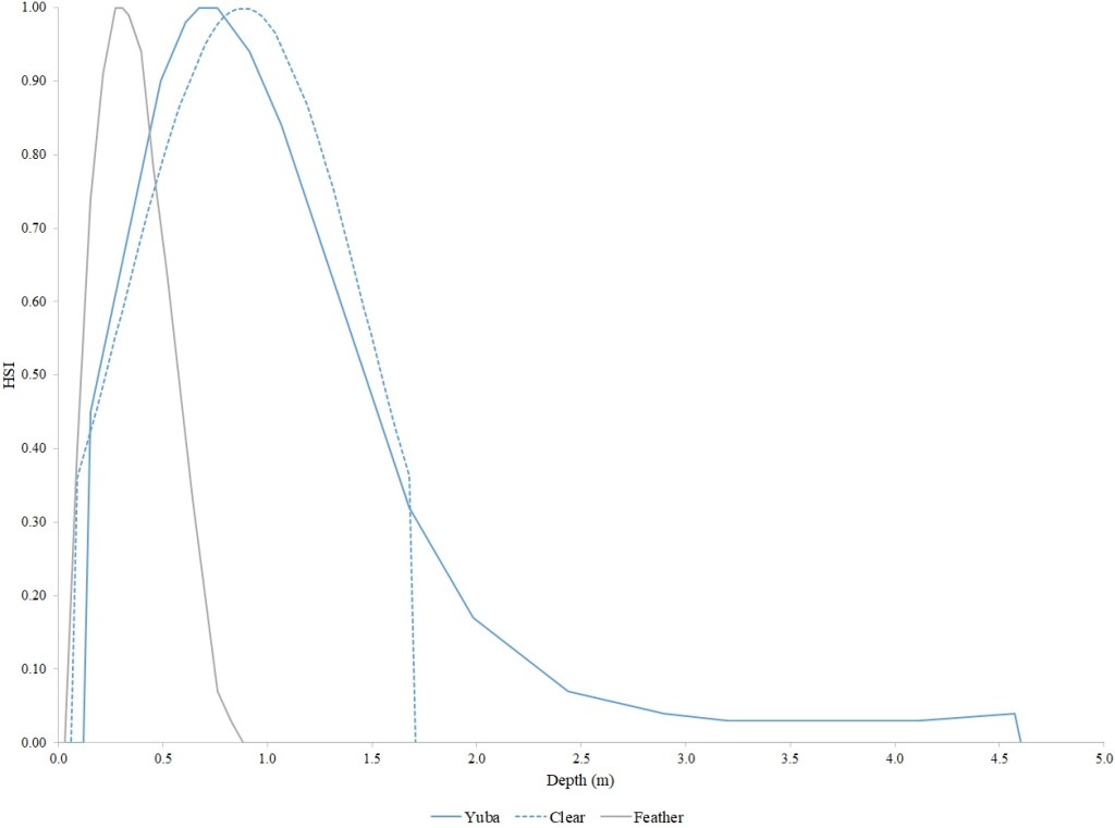
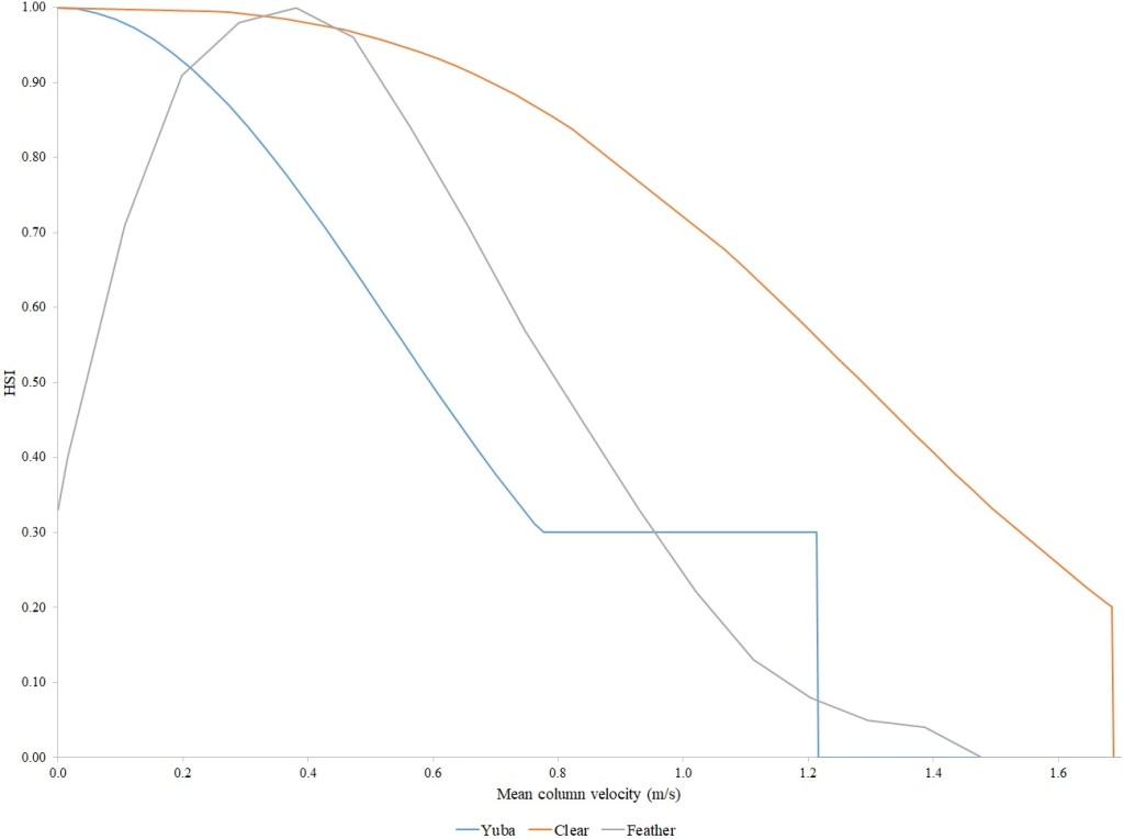
For Chinook Salmon fry rearing, all optimal depths were less than 0.55 m, and all optimal velocities were less than 0.14 m/s. Notably, the two HSC with the highest non-zero depth suitability (Sacramento fall-run and Yuba fall/spring run) were where SCUBA was used to locate fry and juvenile Chinook Salmon in deep water. In contrast, the HSC with highest non-zero velocity suitability was on the Tuolumne River. Cover HSC showed consistent optimal HSI values for complex woody cover (cover codes 4, 4.7, 5, and 5.7) and undercut banks. The Yuba River fall/spring-run Chinook Salmon HSC showed the largest effect of adjacent velocity. There was no adjacent velocity HSC for Clear Creek spring-run Chinook Salmon, since the final step in the development of the HSC produced a relationship in which suitability decreased with increasing adjacent velocity.

Except for the Feather River, all Chinook Salmon juvenile rearing HSC had optimal depths ranging from 0.17–1.07 m. The Feather River Chinook Salmon juvenile rearing HSC had an optimal suitability for all depths greater than 0.274 m. For the remaining criteria, the American and Sacramento rivers HSC had the highest depths with non-zero suitability. Optimal velocities ranged up to 0.38 m/s, while non-zero-suitabilities ranged up to 1.69 m/s (for Clear Creek spring-run Chinook Salmon). Cover criteria for Chinook Salmon juvenile were consistent with those for fry; those for the Sacramento River were the same for both fry and juvenile, since there was no significant difference in the habitat use data between the two life stages for all three runs of Chinook Salmon. There was a larger effect of adjacent velocity for juveniles than for fry.

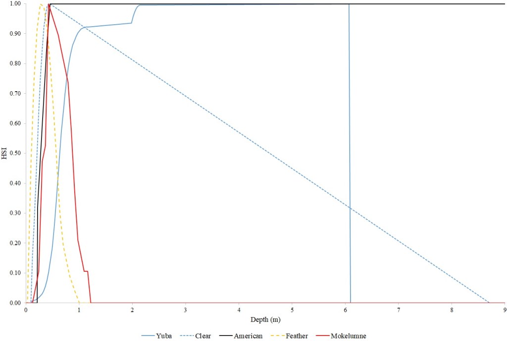
Steelhead spawning depth HSC showed considerable diversity. The Feather River HSC had the shallowest depths, with suitability reaching zero at just over one m. The American River HSC had suitability that stayed at 1.0 for depths greater than 0.46 m, reflecting that the application of the Gard (1998) depth correction methodology did not show a decrease in suitability with increasing depth, with the availability of areas with suitable velocity and substrate decreasing faster than habitat use. The Yuba River HSC had high suitabilities for depths greater than one m. Twenty four percent of the Yuba River steelhead redds had depths greater than 1.52 m, while the deepest redd had a depth of 6.06 m. Optimal velocities ranged from 0.24 m/s for the American to 0.88 m/s for the Yuba and Feather. The Yuba had the highest non-zero suitability at 2.11 m/s. Suitability for substrates were consistently shifted to smaller substrates for steelhead, versus Chinook Salmon. Steelhead consistently had an optimal suitability for substrate code 1.2. Substrate data were not collected for the American River steelhead redds.

Optimal depths for steelhead fry ranged from 0.03 m for Clear Creek to 0.58 m for the Yuba, while the largest non-zero-suitability ranged from 1.22 m for Clear Creek to 1.92 m for the Yuba. For velocities, steelhead fry consistently had near-zero values for optimal suitabilities, while the largest non-zero-suitability ranged from 0.39 m/s for the Feather River to 1.12 m/s for the Yuba. Steelhead fry cover criteria were similar to those for Chinook Salmon. On the Sacramento River, although I did not collect steelhead HSC data, I frequently saw mixed schools of Chinook Salmon and steelhead while I was collecting HSC data for Chinook Salmon. There was a larger effect of adjacent velocity for steelhead fry than for Chinook Salmon fry.

For steelhead juveniles, optimal depths ranged from 0.27 m for the Feather to 0.76 m for the Yuba. Similarly, the highest non-zero-suitability ranged from 0.88 m for the Feather to 4.6 m for the Yuba. Optimal mean column velocities for steelhead juveniles were consistently less than 0.4 m/s, while the highest non-zero-suitability ranged from 1.22 m/s for the Yuba to 1.69 m/s for Clear Creek. Steelhead juvenile criteria were consistent with Chinook Salmon in showing optimal suitabilities for complex woody cover and undercut banks. On Clear Creek both Chinook Salmon and steelhead juveniles showed optimal suitability for cobble. Steelhead juveniles had the largest effect of adjacent velocity of the species and life stages I examined.

Biological verification was successful in ten out of thirteen cases (Table 4). Biological verification was more successful for spawning than for fry and juvenile rearing.

Table 4. Biological verification results for the Habitat Suitability Criteria including stream, species, run, life stage, the median combined suitability for occupied and unoccupied, sample size, and P-value. (NA = Not Applicable)

Stream	Species	Run	Life stage	Suitability – Occupied	Suitability – Unoccupied	n	P-value
Butte	Chinook	spring	spawning	0.18	0.0009	295, 1860	<0.0001
Clear	Chinook	spring	spawning	0.1599	0.0000	7, 719	0.026
Clear	steelhead	NA	spawning	0.0563	0.0008	26, 875	<0.0001
Clear	Chinook	fall	spawning	0.38	0.12	464, 1436	<0.0001
Clear	Chinook	fall	fry	0.33	0.16	73, 127	<0.0001
Clear	Chinook	fall	juvenile	0.13	0.10	29, 165	0.025
Yuba	Chinook	spring	spawning	0.23	0.01	146, 1200	<0.0001
Yuba	Chinook	fall	spawning	0.39	0.11	422, 1600	<0.0001
Yuba	steelhead	NA	spawning	0.245	0.0004	32, 600	<0.0001
Yuba	Chinook	fall /spring	fry	0.094	0.086	33, 52	0.086
Yuba	steelhead	NA	fry	0.036	0.048	71, 98	0.741
Yuba	Chinook	fall /spring	juvenile	0.358	0.011	5, 23	0.013
Yuba	steelhead	NA	juvenile	0.019	0.017	3, 80	0.66

For the meta-analysis, correlations between optimal depths and velocities, and flow and slope, ranged from –0.41–0.56. The only correlation that was statistically significant at P = 0.05 was optimal depth for juvenile versus channel slope. For the Kruskal-Wallis tests, all P-values were greater than 0.05 except for juvenile optimal depth. In that case, where the P-value was 0.008, the median optimal depth was greatest for the presence/absence method (0.85 m) and least for the use method (0.29 m).

Discussion

The meta-analysis was generally inconclusive at explaining why there are differences in HSC across rivers. Differences in the amount or quality of habitat, where fish are using sub-optimal habitat because that is all that is available, only showed significant differences for juvenile rearing depth, where the presence/absence method helped to correct for limited availability of deeper conditions. Similarly, watershed conditions were only significant for juvenile rearing depth versus slope. Higher gradient streams that are more bedrock-dominated generally have a higher proportion of deep pools, and thus higher availability of deeper habitat. Differences in population size, which was not captured in the meta-analysis, may interact with habitat availability. Large population sizes, which have increased intra-species competition, can exacerbate effects of limited habitat availability, as some individuals are forced into sub-optimal habitat conditions. Density dependent effects for fry and juvenile rearing are likely to be greater in the presence of in-river hatchery releases. Streams with large populations of both Chinook Salmon and steelhead, with similar habitat requirements, can have higher density dependent effects through inter-species competition. Differences between streams in juvenile use of deeper habitats may reflect avoidance of habitat where piscine predators are prevalent.

Cases where biological validation was unsuccessful generally resulted in differences between habitat conditions when physical data were collected and when validation occurred, as a result of scour or sediment deposition post surveys. Validation was likely more successful for spawning due to the better ability of hydraulic models to simulate depth and velocity at larger scales (redds versus individual fry and juveniles) and due to larger sample sizes.

Presence/absence methods to develop criteria will generally result in HSC that are less biased due to the effects of availability, and thus should provide better predictions of habitat selection at different flows. In larger rivers, use of underwater video and SCUBA diving were able to identify redds, fry, and juveniles in deeper conditions than could be identified wading or snorkeling. As a result, the US Fish and Wildlife Service HSC for the Yuba River are recommended for evaluating habitat restoration projects on larger rivers, while HSC developed on Clear Creek are recommended for evaluating habitat restoration projects on smaller Central Valley streams. The HSC parameters presented in this paper should be viewed as necessary but not sufficient conditions for habitat restoration projects. For example, water temperature and groundwater upwelling and downwelling are additional considerations for spawning habitat. Conditions that promote flow through spawning gravel, such as the lateral dunes made during Chinook Salmon spawning on the Sacramento River, are also important to consider in designing spawning restoration projects. An important caveat for the HSC presented in this paper is that the data for them were all collected for in-channel conditions. As a result, it is recommended that the fishery benefits of floodplain restoration projects be quantified by the amount of wetted area created.

The HSC presented in this paper have implications for designing restoration projects at multiple spatial scales. For the entire Central Valley, flow-habitat relationships generated from these HSC are a key input to decision support models (Peterson and Duarte 2020) used to set restoration priorities. Within a given stream, limiting life stage analyses from flow-habitat relationships can set priorities for what type of habitat restoration project (spawning versus rearing) can be expected to result in population increases. For example, side channel projects, which can provide optimal depths and velocities for rearing, would be a priority for streams where fry habitat is the limiting life stage. In the early stages of design of a given restoration project, optimal HSC values are useful design parameters. Flow-habitat relationships for existing versus proposed conditions (Gard 2006) can be useful in identifying needed design refinements, such as adding large woody debris. HSC, together with hydraulic modeling, can be used to quantify changes in habitat associated with restoration, as well as changes over time due to high flows (Gard 2014). Adjacent velocity HSC for fry and juvenile rearing can best be incorporated into designs through maximizing topographic complexity, such as alcoves, varying channel widths, and alternating pools and riffles in side channels. For spawning projects, the gravel mix in Icanberry (2006) is recommended, rather than the substrate HSC in this paper, since the inclusion of smaller particles (6 to 12 mm) is critical for egg survival.

Acknowledgements

Mention of specific products does not constitute endorsement by the U.S. Fish and Wildlife Service. The study was funded by the Anadromous Fisheries Restoration Program (Section 3406[b][1]) of the Central Valley Project Improvement Act (Title XXXIV of P.L. 102-575). Thanks to the many people who helped me collect habitat suitability criteria data for the U.S. Fish and Wildlife Service studies cited in this paper, especially Ed Ballard, Rick Williams, Bill Pelle, Erin Strange, and John Kelly.

Literature Cited

• Aceituno, M. E. 1990. Habitat preference criteria for fall-run Chinook Salmon holding, spawning and rearing in the Stanislaus River, California. U.S. Fish and Wildlife Service, Sacramento, CA, USA.
• Ahmadi-Nedushan, B. A., A. St-Hilaire, M. Berube, E. Robichaud, N. Theimonge, and B. Bobee. 2006. A review of statistical methods for the evaluation of aquatic habitat suitability for instream flow assessment. River Research and Applications 22:503–523.
• Bovee, K. D. 1978. Probability-of-use criteria for the family Salmonidae. Instream Flow Information Paper No. 4. Cooperative Instream Flow Service Group, U.S. Fish and Wildlife Service, Fort Collins, CO, USA.
• Bovee, K. D., B. L. Lamb, J. M. Bartholow, C. B. Stalnaker, J. Taylor, and J. Henriksen. 1998. Stream habitat analysis using the instream flow incremental methodology. Biological Resources Division Information and Technology Report USGS/BRD-1998-0004. U.S. Geological Survey, Biological Resource Division, Dixon, CA, USA.
• Beak Consultants, Inc. 1989. Yuba River fisheries investigations, 1986–1988. Appendix B. The relationship between stream discharge and physical habitat as measured by weighted useable area for fall-run Chinook Salmon (Oncorhynchus tshawytscha) in the lower Yuba River, California. Prepared for State of California Resources Agency, Department of Fish and Game, Sacramento, CA, USA.
• East Bay Municipal Utility District (EBMUD). 2019. Lower Mokelumne River habitat suitability criteria. East Bay Municipal Utility District, Lodi, CA, USA.
• Envirosphere Company. 1991. Lower Mokelumne River fisheries study. Prepared for California Department of Fish and Game, Sacramento, CA, USA.
• Fausch, K. D., and R. J. White. 1981. Competition between Brook Trout (Salvelinus fontinalis) and Brown Trout (Salmo trutta) for positions in a Michigan stream. Canadian Journal of Fisheries and Aquatic Sciences 38:1220–1227.
• Filipe, A., I. Cowx, and M. Collares-Pereira. 2002. Spatial modeling of freshwater fish in semi-arid river systems: a tool for conservation. River Research and Applications 18:123–136.
• Gard, M. 1998. Technique for adjusting spawning depth habitat utilization curves for availability. Rivers 6:94–102.
• Gard, M. 2006. Modeling changes in salmon spawning and rearing habitat associated with river channel restoration. International Journal of River Basin Management 4(3):201–211.
• Gard, M. 2014. Modeling changes in salmon habitat associated with river channel restoration and flow-induced channel alterations. River Research and Applications 30:40–44.
• Gard, M., and E. Ballard. 2003. Applications of new technologies to instream flow studies in large rivers. North American Journal of Fisheries Management 23:1114–1125.
• Geist, D. R., J. Jones, C. J. Murray, and D. D. Dauble. 2000. Suitability criteria analyzed at the spatial scale of redd clusters improved estimates of fall Chinook Salmon (Oncorhynchus tshawytscha) spawning habitat use in the Hanford Reach, Columbia River. Canadian Journal of Fisheries and Aquatic Sciences 57:1636–1646.
• Goodman, D. H., N. Som, and N. J. Hetrick. 2018. Increasing the availability and spatial variation of spawning habitats through ascending baseflows: ascending baseflows and spawning habitats. River Research and Applications 2018:1–10.
• Guay, J. C., D. Boisclair, D. Rioux, M. LeClerc, M. Lapointe, and P. Legendre. 2000. Development and validation of numerical habitat models for juveniles of Atlantic Salmon (Salmo salar). Canadian Journal of Fisheries and Aquatic Sciences 57:2065–2075.
• Hirzel, A. H., and G. Le Lay. 2008. Habitat suitability modeling and niche theory. Journal of Applied Ecology 45:1372–1381.
• Icanberry, J. 2006. Anadromous Fish Restoration Program recommended gravel specifications for spawning habitat restoration projects. U.S. Fish and Wildlife Service, Stockton, CA, USA.
• Knapp, R. A., and H. K. Preisler. 1999. Is it possible to predict habitat use by spawning salmonids? A test using California golden trout (Oncorhynchus mykiss aguabonita). Canadian Journal of Fisheries and Aquatic Sciences 56:1576–1584.
• Manly, B .F. J., L. L. McDonald, D. L. Thomas, T. L. McDonald, and W. P. Erickson. 2002. Resource Selection by Animals, Statistical Design and Analysis for Field Studies. Second Edition. Kluwer Academic Publishers, Dordrecht, Netherlands.
• McHugh, P., and P. Budy. 2004. Patterns of spawning habitat selection and suitability for two populations of spring Chinook Salmon, with an evaluation of generic verses site-specific suitability criteria. Transactions of the American Fisheries Society 133:89–97.
• Parasiewicz, P. 1999. A hybrid model–assessment of physical habitat conditions combining various modeling tools. In: Proceedings of the Third International Symposium on Ecohydraulics, Salt Lake City, UT, USA.
• Pearce, J., and S. Ferrier. 2000. Evaluating the predictive performance of habitat models developed using logistic regression. Ecological Modelling 133(3):225–245.
• Peterson, J. T., and A. Duarte. 2020. Decision analysis for greater insights into the development and evaluation of Chinook Salmon restoration strategies in California’s Central Valley. Restoration Ecology 28(6):1596–1609.
• South Sutter Water District. 2018. Application for new license, major project – existing dam, Volume II: Exhibit E – Environmental report, Camp Far West Hydroelectric Project, FERC Project No. 2997. South Sutter Water District, Trowbridge, CA, USA.
• Thomas R. Payne and Associates. 1995. Battle Creek instream flow study, specified fisheries investigations on Battle Creek, Shasta, and Tehama Counties. Prepared for California Department of Fish and Game, Redding, CA, USA.
• Thomas R. Payne and Associates. 2002. Oroville Facilities Relicensing (Project No. 2100) SP-F16 Evaluation of project effects on instream flows and fish habitat, draft phase 1 report. Prepared for Oroville Facilities Relicensing Environmental Work Group, Oroville, Ca, USA.
• Thomas, J. A., and K. D. Bovee. 1993. Application and testing of a procedure to evaluate transferability of habitat suitability criteria. Regulated Rivers: Research and Management 8:285–294.
• Tiffan, K. E., R. D. Garland, and D. W. Rondorf. 2002. Quantifying flow-dependent changes in sub-yearling fall Chinook Salmon rearing habitat using two-dimensional spatially explicit modeling. North American Journal of Fisheries Management 22:713–726.
• Tirelli, T., L. Pozzi, and D. Pessani. 2009. Use of different approaches to model presence/absence of salmon marmoratus in Piedmont (northwestern Italy). Ecological Informatics 4:234–243.
• U.S. Fish and Wildlife Service (USFWS). 1985. Flow needs of Chinook Salmon in the lower American River. Final report on the 1981 lower American River flow study. U.S. Fish and Wildlife Service, Sacramento, CA, USA.
• U.S. Fish and Wildlife Service (USFWS). 1994. The relationship between instream flow and physical habitat availability for Chinook Salmon in the Lower Tuolumne River, California. U.S. Fish and Wildlife Service, Sacramento, CA, USA.
• U.S. Fish and Wildlife Service (USFWS). 1997a. Supplemental report on the instream flow requirements for fall-run Chinook Salmon spawning in the Lower American River. U.S. Fish and Wildlife Service, Sacramento, CA, USA.
• U.S. Fish and Wildlife Service (USFWS). 1997b. Identification of the instream flow requirements for fall-run Chinook Salmon spawning in the Merced River. U.S. Fish and Wildlife Service, Sacramento, CA, USA.
• U.S. Fish and Wildlife Service (USFWS). 2003. Flow-habitat relationships for steelhead and fall, late-fall, and winter-run Chinook Salmon spawning in the Sacramento River between Keswick Dam and Battle Creek. U.S. Fish and Wildlife Service, Sacramento, CA, USA.
• U.S. Fish and Wildlife Service (USFWS). 2005a. Flow-habitat relationships for spring-run Chinook Salmon spawning in Butte Creek. U.S. Fish and Wildlife Service, Sacramento, CA, USA.
• U.S. Fish and Wildlife Service (USFWS). 2005b. Flow-habitat relationships for Chinook Salmon rearing in the Sacramento River between Keswick Dam and Battle Creek. U.S. Fish and Wildlife Service, Sacramento, CA, USA.
• U.S. Fish and Wildlife Service (USFWS). 2006. Flow-habitat relationships for spring-run Chinook Salmon and steelhead/rainbow trout spawning in Clear Creek between Whiskeytown Dam and Clear Creek Road. U.S. Fish and Wildlife Service, Sacramento, CA, USA.
• U.S. Fish and Wildlife Service (USFWS). 2010a. Flow-habitat relationships for spring and fall-run Chinook Salmon and steelhead/rainbow trout spawning in the Yuba River. U.S. Fish and Wildlife Service, Sacramento, CA, USA.
• U.S. Fish and Wildlife Service (USFWS). 2010b. Flow-habitat relationships for juvenile fall/spring-run Chinook Salmon and steelhead/rainbow trout rearing in the Yuba River. U.S. Fish and Wildlife Service, Sacramento, CA, USA.
• U.S. Fish and Wildlife Service (USFWS). 2011a. Flow-habitat relationships for juvenile spring-run Chinook Salmon and steelhead/rainbow trout rearing in Clear Creek between Whiskeytown Dam and Clear Creek Road. U.S. Fish and Wildlife Service, Sacramento, CA, USA.
• U.S. Fish and Wildlife Service (USFWS). 2011b. Flow-habitat relationships for fall-run Chinook Salmon and steelhead/rainbow trout spawning in Clear Creek between Clear Creek Road and the Sacramento River. U.S. Fish and Wildlife Service, Sacramento, CA, USA.
• U.S. Fish and Wildlife Service (USFWS). 2013. Flow-habitat relationships for juvenile spring-run and fall-run Chinook Salmon and steelhead/rainbow trout rearing in Clear Creek between Clear Creek Road and the Sacramento River. U.S. Fish and Wildlife Service, Sacramento, CA, USA.
• Vogel, D. A. 1982. Preferred spawning velocities, depths and substrates for fall Chinook Salmon in Battle Creek, California. U.S. Fish and Wildlife Service, Red Bluff, CA, USA.

Appendices for “Central Valley anadromous salmonid habitat suitability criteria”