FULL RESEARCH ARTICLE

Juan Antonio Maldonado-Coyac¹, Dana Isela Arizmendi-Rodríguez², Rebeca Sánchez-Cárdenas¹, Marcela Selene Zúñiga-Flores³, Maria de los Angeles Maldonado-Amparo¹, Manuel Otilio Nevárez-Martínez², and Luis Antonio Salcido-Guevara¹*

¹ Universidad Autónoma de Sinaloa, Paseo Claussen, Mazatlán, Sinaloa, México
 https://orcid.org/0000-0001-6535-0405 (JAMC)
https://orcid.org/0000-0001-9568-8757 (RSC)
 https://orcid.org/0000-0003-3005-9348 (MAMA)
 https://orcid.org/0000-0003-1608-8986 (LASG)
² Instituto Mexicano de Investigación en Pesca y Acuacultura Sustentables (IMIPAS), Guaymas, Sonora, México
 https://orcid.org/0000-0003-4698-2735 (DIAR)
 https://orcid.org/0000-0002-4661-3246 (MONM)
³ Instituto Politecnico Nacional Centro Interdisciplinario de Ciencias Marinas, Playa Palo Santa Rita 23096, La Paz, Baja California Sur, México
 https://orcid.org/0000-0003-0797-1961 (MSZF)

*Corresponding Author: lsalcido@uas.edu.mx

Published 22 May 2026 • doi.org/10.51492/cfwj.112.7

Abstract

Relative growth and body condition of the Finescale Triggerfish (Balistes polylepis) were evaluated using fishery-dependent data from the southeastern Gulf of California across eight sampling periods between 2002 and 2024. Growth consistently showed a negative allometric pattern, with marked ontogenetic shifts occurring within a narrow size range closely associated with sexual maturity and likely changes in habitat use. These growth transitions indicate reallocation of energy from somatic development toward reproduction. The condition factor varied significantly among periods but generally remained close to unity, indicating good overall physiological status of the population. Although lower condition values coincided with the extreme El Niño event of 2015–2016, the association between climatic anomalies and body condition was not statistically significant, suggesting broad resilience to regular environmental variability and potential sensitivity only during extreme events. These results highlight the importance of accounting for ontogenetic growth shifts when assessing population dynamics and provide ecological insight relevant for the management of this exploited species.

Key words: allometry, Balistes polylepis, condition factor, El Niño-Southern Oscillation, fisheries management, Gulf of California, relative growth, reproduction investment, sexual maturity

Citation: Maldonado-Coyac, J. A., D. I. Arizmendi- Rodríguez, R. Sánchez-Cárdenas, M. S. Zúñiga-Flores, M. Maldonado-Amparo1, M. O. Nevárez-Martínez, and L. A. Salcido-Guevara. 2026. Relative growth and condition factor of the Finescale Triggerfish in the southeastern Gulf of California. California Fish and Wildlife Journal 112:e7.

Editor: Elyse Freitas, Fisheries Branch

Submitted: 2 November 2025; Accepted: 6 January 2026

Copyright: ©2026, Maldonado-Coyac et al. This is an open access article and is considered public domain. Users have the right to read, download, copy, distribute, print, search, or link to the full texts of articles in this journal, crawl them for indexing, pass them as data to software, or use them for any other lawful purpose, provided the authors and the California Department of Fish and Wildlife are acknowledged.

Competing Interests: The authors have not declared any competing interests.

Introduction

Finescale Triggerfish (Balistes polylepis Steindachner 1876) belongs to the Family Balistidae and the Order Tetraodontiformes, and it is found from northern California to the Gulf of California (GC), Chile, and the oceanic islands of Hawaii, Galapagos, and Marquesas(Froese and Pauly 2023; Robertson and Allen 2024). It inhabits rocky reefs, slopes and adjacent sandbanks, at depths of 3 to 512 m (Robertson and Allen 2024), where it feeds mainly on invertebrates and marine algae (Acosta-Pachón et al. 2023) and regulates populations of sea urchins, crustaceans and molluscs (Humann and Deloach 1993). B. polylepis reproduction is closely associated with the demersal environment, where males form nests for the incubation of eggs that are kept under the close care of the female, while the male scares away other males and potential predators (Strand 1978; De la Cruz-Agüero et al. 1997), which occurs during the months of May to October in some areas of the Gulf of California (Ontiveros-García 2005; García-Pérez 2019). Once the eggs hatch, their larvae and juvenile stages are pelagic, and they become demersal upon reaching adulthood (Eschmeyer et al. 1983).

B. polylepis is a species that reaches a size of 76 cm in total length (TL) (Eschmeyer et al. 1983) and an estimated longevity of up to 21 years (Valdez-Ornelas et al. 2007). According to the available information, the relative growth of B. polylepis described from the potential relationship between length and weight (LWR, Ricker 1975; Froese 2006) has been defined mainly as negative allometric or hypoallometric and presents a wide variation in the allometry coefficient (b) with values from 1.79 to 2.71 among the different study areas (Table 1). This indicates that larger specimens change their body shape, becoming more elongated, or that smaller specimens exhibit a better condition at the time of sampling (Froese 2006). Only López-Martínez et al.(2012) have reported isometric growth for B. polylepis along the coasts of Nayarit, Sinaloa, and Sonora, which means that the small specimens in the sample had the same shape and condition as the large specimens (Froese 2006), and the latter with greater robustness with respect to those with hypoallometric growth in other areas and periods (Table 1). In other species, such as B. capriscus, B. vetula, Odonus niger, Pseudobalistes fuscus, Rhinecanthus aculeatus, Sufflamen fraenatum, Xanthichthys ringens, a variable trend in relative growth between different zones has also been observed (Table 1). These variations may be due to several factors, such as the time of year, stomach filling, sex, degree of development of gonads, size and number of organisms used for the analysis (Ricker 1975; Froese 2006), but they could also be variations between populations in response to the ecological conditions of the habitat in each area or period (Erisman et al. 2021). However, the trend among species of the Balistidae family is the dominance of negative allometric growth but with notable variations (Table 1), which suggests that relative growth is sensitive or plastic in response to environmental variability (Karjalainen et al.2016). In turn, these variations indicate variations in the nutritional condition of individuals in different populations and/or over time (Le Cren 1951; Froese 2006), which in turn has important implications for different biological processes, for example impacting individual growth rates (Dutta 1994), the quality and quantity of egg production (Volkoff and London 2018), the onset of sexual maturity (Ricker 1975; Froese 2006; Fontoura et al. 2010), population biomass (Bhukaswan 1980), etc. All the implications are crucial aspects to consider in fisheries management, conservation, aquaculture or any use or service involving these species (Ricker 1975; Bhukaswan 1980; Froese 2006; Erismanet al. 2021), and the study of relative growth provides relevant information, for example, only from an updated LWR it is possible to estimate the biomass of the catches from simple size data (e.g., total length), which is essential to regulate catches (Froese et al. 2014).

Table 1. Sizes and parameters of the length-weight relationships (LWR, power model) of Balistidae species reported around the world. * indicates significant differences between the hypothetical isometry value (b = 3); TL = total length; FL = furcal length; SL = standard length; NA = data not available.

Species	n	Sex	Size Min–Max	LWR a	LWR b	Study Area	References
Abalistes stellatus	NA	Unsexed	14–53.5 FL	0.0603	2.692*	New Caledonia	Letourneur et al. 1998
Balistes polylepis	552	Both sexes	16–53 TL	0.0547	2.7*	Mazatlán, Mexico	Barroso-Soto et al. 2007
Balistes polylepis	62	Both sexes	30.2–47.0 TL	NA	1.79*	Bahía de los Ángeles, Baja California Sur, Mexico	Valdez-Ornelas et al. 2007
Balistes polylepis	1,696	Both sexes	3.5–32.5 TL	0.00007	2.7338	Gulf of California, Mexico	López-Martínez et al. 2012
Balistes polylepis	433	Both sexes	17–48 TL	0.0833	2.5159*	San Cosme to Punta Coyote corridor, Baja California Sur, Mexico	Yee-Duarte et al. 2018
Balistes polylepis	101	Both sexes	5.8–31 TL	0.042	2.701*	Bahía Magdalena-Almejas Lagoon System, Baja California Sur, Mexico	Rábago-Quiroz et al. 2017
Balistes polylepis	79	Both sexes	5.2–42.8 TL	0.043	2.71*	Southern Sinaloa to Northern Nayarit, Mexico	Nieto-Navarro et al. 2010
Balistes capriscus	814	Males	15.3–34.7 FL	0.000005	3.265*	São Paulo, Brazil	Bernardes 2002
Balistes capriscus	1,240	Females	19.9–33.4 FL	0.000003	3.34*	São Paulo, Brazil	Bernardes 2002
Balistes capriscus	2,054	Both sexes	16–23 FL	0.000004	3.299*	São Paulo, Brazil	Bernardes 2002
Balistes capriscus	271	Males	11.9–44.6 FL	0.0215	3.046*	Gulf of Gabés, Mediterranean	Kacem et al. 2015
Balistes capriscus	480	Females	11.3–44.5 FL	0.041	2.835*	Gulf of Gabés, Mediterranean	Kacem et al. 2015
Balistes capriscus	751	Both sexes	11.3–44.6 FL	0.0324	2.915*	Gulf of Gabés, Mediterranean	Kacem et al. 2015
Balistes capriscus	12	Unsexed	6.5–22.5 TL	0.0176	3.0548	Caribbean Sea, French West Indies	Mahé et al. 2023
Balistes vetula	18	Both sexes	19.5–43.5 FL	0.0518	2.81*	Gulf of Salamanca, Colombia	García et al. 1998
Balistes vetula	<649	Both sexes	18–46 FL	0.00004	2.95	Brazil Coast	Albuquerque et al. 2011
Balistes vetula	107	Unsexed	21.5–66 TL	0.1758	2.2849*	Caribbean Sea, French West Indies	Mahé et al. 2023
Balistapus undulatus	22	Unsexed	6.5–19 SL	0.0565	2.947	Philippines, Davao Gulf	Gumanao et al. 2016
Balistoides viridescens	12	Unsexed	4.9–26.5 SL	0.0696	2.929	Philippines, Davao Gulf	Gumanao et al. 2016
Canthidermis sufflamen	19	Unsexed	36.5–57.5 TL	0.1583	2.2849*	Caribbean Sea, French West Indies	Mahé et al. 2023
Melichthys niger	62	Unsexed	15–31.5 TL	0.0570	2.7445*	Caribbean Sea, French West Indies	Mahé et al. 2023
Odonus niger	257	Males	15.5–24 TL	0.046	2.565*	India, Karnataka coast	Suyani et al. 2021
Odonus niger	101	Females	15.4–23 TL	0.044	2.589*	India, Karnataka coast	Suyani et al. 2021
Odonus niger	358	Both sexes	15.4–24 TL	0.047	2.561*	India, Karnataka coast	Suyani et al. 2021
Odonus niger	13	Unsexed	13–19.5 SL	0.0438	2.91	Philippines, Davao Gulf	Gumanao et al. 2016
Pseudobalistes fuscus	NA	Unsexed	26–57 FL	0.2318	2.452*	New Caledonia	Letourneur et al. 1998
Rhinecanthus aculeatus	352	Both sexes	2–20.9 SL	0:000097	2.834*	Japan, Okinawa Island	Künzli and Tachihara 2012
Sufflamen fraenatum	NA	Unsexed	19–36.5 TL	0.031	2.95	New Caledonia	Letourneur et al. 1998
Xanthichthys ringens	13	Unsexed	14.5–19.5 TL	0.4983	1.912*	Caribbean Sea, French West Indies	Mahé et al. 2023

In northwestern Mexico, approximately 50% of Mexican fishery production is extracted (Cisneros-Mata et al. 2010), which is made up of around 136 fishery resources. Where B. polylepis is an important resource, which is fished mainly by artisanal fishing and secondarily by industrial fishing (DOF 2010; Díaz-Uribe et al. 2013), using fishing gear such as handlines with hooks (Barroso-Soto et al. 2007), seine nets, traps, longlines, (García-Pérez 2019; González-Cuellar et al. 2019), demersal scale trawls (INAPESCA 2000) and incidentally with shrimp trawls (INAPESCA 2000; López-Martínez et al. 2012). For much of the year, this fishery is an important source of food and employment for the coastal communities of the Gulf of California (Barroso-Soto et al. 2007; Erisman et al. 2010; López-Martínez et al. 2012), with a growing fishing production exceeding 5,500 tons per year (Saucedo-Barrón and Ramírez-Rodríguez 1994; Erismanet al. 2010; González-Cuellar et al. 2019), although this data could be underestimated since there are no specific records of all landing sites. In this context, there is a constant interaction between the fishery and the populations of B. polylepis, and consequently, with all aspects of its life history (Ontiveros-García 2005; López-Martínez et al. 2012; García-Pérez 2019); however, the impacts are unknown. Therefore, it is necessary to have biological information on this species, as well as indicators of the status and dynamics of its populations over time, for the implementation of appropriate management measures for the regulation of its fishery throughout its distribution (López-Martínez et al. 2012). This is often challenging due to the scarce biological data and systematic records per species, or best, per exploited populations (McCarthy 2012; Sagarese et al. 2018). In Mexico, the available information in official records, such as the National Fisheries Charter and the Statistical Yearbook of Aquaculture and Fisheries, is grouped by “resource”, a category made up of a variable number of species (DOF 2010; CONAPESCA 2018). Usually, the grouped species belong to the same family.

In this context, an analysis of the relative growth of B. polylepis was conducted, initially based on the LWR (Ricker 1975; Froese 2006) and the relative condition factor (Le Cren 1951), using data from eight discrete sampling periods between 2002 and 2024. Given the high energetic cost associated with nesting and parental care (Strand 1978; Smith and Wootton 1995), potential inflection points in relative growth during the ontogenetic transition from juvenile to adult were evaluated using the broken-stick (BS) and two-segment (TS) models, both of which have been successfully applied for this purpose in recent studies (Katsanevakis et al. 2007; Rabaoui et al. 2007; Rodríguez-Domínguez et al. 2018).

Accordingly, we hypothesized that (1) relative growth exhibits a change point associated with sexual maturity, and (2) individual condition varies in relation to large-scale climatic anomalies. To address the second hypothesis, an exploratory analysis was conducted to evaluate the association between relative condition and temperature anomalies related to the El Niño–Southern Oscillation (ENSO), which includes cold (La Niña) and warm (El Niño) phases in the tropical Pacific (Huang et al. 2017; NOAA 2024). Together, these analyses aim to improve our understanding of how ontogenetic transitions and broad-scale environmental variability may influence relative growth patterns in B. polylepis.

Methods

Data Collection

We collected samples from commercial catches of the artisanal fishery operating at the landing site at Playa Norte, Mazatlan, Sinaloa, Mexico (23.208 N 106.424 W), between 2002 and 2024. Fish were captured using handlines equipped with 11/0 and 12/0 hooks aboard small artisanal wooden boats locally known as Cayucos, measuring 5 to 7 m in length and coated with fiberglass. These vessels have a load capacity of 500 kg and are powered by 16 hp Briggs and Stratton stationary engines. They are also equipped with fish tanks that provide a constant exchange of seawater, allowing for post-harvest preservation until landing and marketing by the same authorized fishermen.

Sampling was fishery-dependent and opportunistic, resulting in uneven temporal coverage. Sampling periods represent discrete collection windows rather than a continuous time series. We retained early and infrequent sampling events because they expanded the size and weight range required for growth and maturity analyses. Sampling gaps, particularly between 2019 and 2021, were largely due to external constraints associated with the COVID-19 pandemic rather than changes in population availability.

Biometry measurements, including total length (TL, ± 0.1 cm) and total weight (TW, ± 0.1 g), were obtained from 3,260 specimens of B. polylepis. We determined sex for approximately 43% of the individuals, reflecting the fishery-dependent nature of the data and the fact that specimens were not consistently processed at the landing site across all sampling periods (Table 2).

Length-Weight Relationship

Relative growth was described from the LWR for each sampling period and for the total data (Table 2), using the power model:

TW = aTL^b

Where a is the shape parameter (intercept) and b is the allometry coefficient (slope) (Froese 2006); where if b = 3, relative growth is isometric, but if b < 3 it is negative allometric (hypoallometric), and if b > 3 it is positive allometric (hyperallometric) (Froese 2006; Froese et al. 2011). Prior to model fitting, we included all individuals with complete TL and TW measurements, whereas specimens with missing or unreliable biometric data were excluded. Following recommendations for evaluating LWR (Froese 2006), we plotted ln(TW) against ln(TL) to visually identify potential outliers. We removed observations showing implausible length–weight combinations, likely associated with measurement or recording errors, from the analyses. Only a very small number of records were excluded, and their removal did not affect the overall conclusions.

Table 2. Sampling periods with available biometric data of Balistes polylepis (TL, ± 0.1 cm; TW, ± 0.1 g) and number of specimens collected. “Both sexes” represents the sum of males and females within each sampling period and does not constitute an independent dataset. These values are shown for reference only.

Season	Sampling Period	Data Category	Number of Specimens
1	Mar to Apr 2002	Unsexed	78
2	Jan 2004 to Feb 2005	Males	270
2	Jan 2004 to Feb 2005	Females	294
2	Jan 2004 to Feb 2005	Both sexes	564
3	Sep 2015 to Aug 2016	Unsexed	382
4	Sep 2016 to Mar 2017	Unsexed	515
5	Sep 2018 to Sep 2019	Unsexed	684
6	Aug 2021 to Jul 2022	Males	208
6	Aug 2021 to Jul 2022	Females	255
6	Aug 2021 to Jul 2022	Both sexes	463
7	Aug 2022 to Aug 2023	Males	196
7	Aug 2022 to Aug 2023	Females	177
7	Aug 2022 to Aug 2023	Both sexes	373
8	Apr to Dec 2024	Unsexed	201
—	Grouped data	—	3,260

We fitted the model to natural log-transformed TL and TW data, assuming additive error in the log-transformed scale, with normally distributed residuals and constant variance, and parameters were estimated by maximizing the log-likelihood objective function using a Newton-based optimization algorithm (Neter et al. 1996).

Where LL is the log-likelihood, Ø is a model parameter, n is the sample size, n is the total body weight, and TW_i is the estimated total weight. Due to the interdependence between the parameters a and b in the power model (Froese 2006), the variation in a was constrained to values < 0.1 during model fitting.

The relative condition factor (Kn) was estimated for each season using the equation proposed by Le Cren (1951): Kn = (TW)/(aTL^b) , where TW and TL are previously defined variables, while a and b are the parameters of the LWR (Froese 2006) adjusted from the total data.

We estimated the confidence intervals (CIs) for parameters (a and b of the LWR) and the Kn per data set as ± [1.96*(SE)] (Zar 2010). A Student´s t-test was used (Zar 2010) to compare slopes (b) of LWR per sampling period and sexes and to define the type of relative growth (whether b = 3, > 3, or < 3). We performed a one-way analysis of variance (ANOVA) and Tukey´s post-hoc test using Statistica 7.0 software (StatSoft) to evaluate differences in Kn among sampling periods.

Identification of Relative Growth Stanzas

We explored the relative growth stanzas for each sampling period by broken-stick models (BS), that were fitted as ln(TW) = lna₁ + b₁ln(TL)if TL ≤ B or or ln(TW) = lna₁ + (b₁ – b₂)ln(B) + b₂Ln(TL) if TL > B; and two-segment models (TS), ln(TW) = lna₁ + b₁ln(TL) if TL ≤ B or ln(TW) = lna₂ + b₂ln(TL) if TL > B. Broken-stick and two-segment models were fitted to log-transformed data using the same maximum-likelihood framework as the power model, allowing the allometry coefficient (b) to take different constant values on either side of the breakpoint (B) (Katsanevakis et al. 2007; Rodríguez-Domínguez et al. 2018).

Whereas the BS and TS models assume a marked morphological change at a specific size of TL = B; the BS represents two straight line segments with different slopes that intersect at TL = B, while the TS represents two straight line segments that do not intersect; therefore, there is a discontinuity point at TL = B, and the slope of the two segments (i.e., b) may or may not be equal (Rabaoui et al. 2007).

For the selection of the model that best describes relative growth stanzas, we used the small-sample bias-corrected form of the Akaike Information Criterion (AICc) (Akaike 1973; Burnham and Anderson 2002). We selected the model with the smallest AIC_c value as the best among the two candidate models. The differences (∆_i) between the AIC_ci of each model and the AIC_cmin of the best model were then determined. According to Burnham and Anderson (2002), models with ∆_i > 10 have essentially no support and could be omitted from further consideration, models with ∆_i < 2 have substantial support, while there is considerably less support for models with 4 < ∆_i < 7. The plausibility of each model, given the data and the two models, was quantified from the Akaike weight (W_i) that is considered to be the weight of evidence in favor of model i from the set of available models (Akaike 1973; Burnham and Anderson 2002).

We calculated the mean length at which fish of a given population become sexually mature for the first time (L_m) for each sampling period using the empirical equations proposed by Froese and Binohlan (2000) as follows: L_∞ = 10^[0.044 + 0.9841 x Log(L_max)]; all data data L_m = 10^[0.8979 x Log(L_∞) – 0.0782], only females L_m = 10^[09469 x Log(L_∞) – 0.1162]; and only males L_m = 10^[09815 X Log(L_∞) – 0.1032]; where L_max is the maximum TL recorded in each sampling period. These L_m, as well as the L₅₀-range (30–32 cm) reported by Ontiveros-García (2005), were compared with the breaking points (ln(B)) obtained from the BS and TS models, under the assumption that the reproduction entails a high energetic cost that may influence the body growth pattern of B. polylepis (Smith and Wootton 1995). For this, breaking points were converted to units of centimeters (cm) using the exponential function (e^ln(B)), and then a Wilcoxon signed-rank test was applied for statistical comparison between empirical L_m and B values (Zar 2010).

Additionally, we explored the association between the El Niño-Southern Oscillation (ENSO) and Kn using the data of Oceanic Niño Index (ONI), calculated as three-month running mean sea surface temperature anomalies for the Niño 3.4 region (5 N–5 S, 120–170 W) (Huang et al. 2017).

We calculated mean ONI values for each sampling period by averaging ONI values corresponding to the months included in each sampling window. These period-specific ONI averages were used to characterize ENSO conditions. We quantified the association between ENSO variability and relative condition using Spearman’s rank correlation between mean Kn and mean ONI values. This analysis was treated as exploratory due to the limited number of sampling periods and uneven temporal coverage. ENSO phases were interpreted using standard thresholds (ONI ≥ +0.5 °C for El Niño, ONI ≤ −0.5 °C for La Niña, and −0.5 °C < ONI < +0.5 °C for neutral conditions) (NOAA 2024).

Results

Length-Weight Relationship

The biometrics of Balistes polylepis recorded from commercial catches off Mazatlan, southeast Gulf of California, during the sampling periods between 2002 and 2024 (Fig. 1) ranged from 16 to 58 cm in total length and from 45 to 3,065 g in total weight (Table 3). We fitted the LWRs for the eight sampling periods with values of a and b, from 0.027 to 0.100 and from 2.496 to 2.871, respectively (Fig. 2, Table 3). The slope analysis (b) indicated that the relative growth was negative allometric in most periods, and only in the first season was isometric growth (P>0.05; Table 3). Also, the b value of the general LWR (grouped data) indicated negative allometric growth (Table 3).

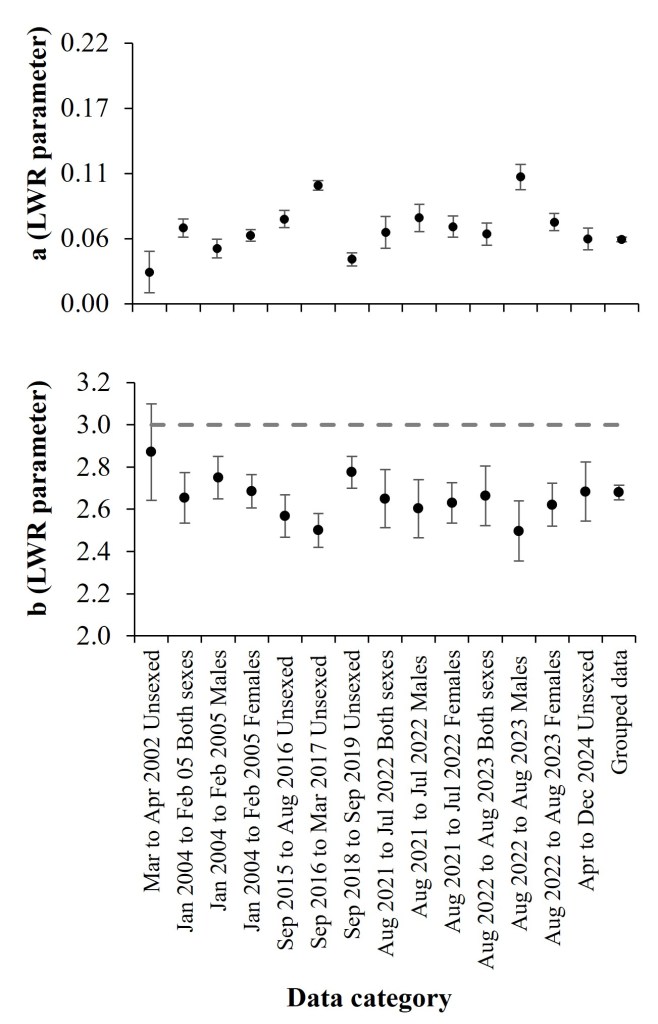
Table 3. Parameters of the length-weight relationship of B. polylepis from off Mazatlán, southeast Gulf of California, during sampling periods from 2002 to 2024. The values ​​of the intercept (a), allometry coefficient (b), confidence intervals (CI) are described, and the asterisk indicates significant differences (P < 0.05) of b with respect to the hypothetical value of b = 3.

Season	Data Category	TL (cm)	TW (g)	LWR a (CI95%)	LWR b (CI95%)	t	P
1	Unsexed	21.4–44	200–1,300	0.027 (0.009–0.044)	2.871 (2.642–3.099)	1.37	0.17
2	Males	17.5–53.5	120–2,600	0.064 (0.056–0.072)	2.654* (2.534–2.774)	21.00	< 0.001
2	Females	16–49.5	120–2,020	0.047 (0.039–0.055)	2.750* (2.630–2.870)	5.02	< 0.001
2	Both sexes	16–53.5	120–2,600	0.058 (0.053–0.063)	2.6842* (2.606–2.763)	27.20	< 0.001
3	Unsexed	16.3–49.5	45–1,935	0.072 (0.064–0.079)	2.568* (2.467–2.669)	19.68	< 0.001
4	Unsexed	20–47	100–1,735	0.100 (0.096–0.104)	2.501* (2.414–2.587)	25.21	< 0.001
5	Unsexed	16.5–51.2	80–2,120	0.038 (0.032–0.043)	2.776* (2.700–2.851)	16.24	< 0.001
6	Males	18.3–49.6	129.9–1,860	0.060 (0.047–0.073)	2.650* (2.465–2.740)	30.19	< 0.001
6	Females	18.5–43.8	150–1,490	0.073 (0.061–0.084)	2.603* (2.465–2.740)	10.62	< 0.001
6	Both sexes	18.3–49.6	129.9–1,860	0.065 (0.056–0.074)	2.629* (2.534–2.725)	41.97	< 0.001
7	Males	21.7–49.2	220–2,110	0.059 (0.050–0.068)	2.664* (2.522–2.805)	8.07	< 0.001
7	Females	20.5–44.8	205–1,390	0.107 (0.096–0.118)	2.497* (2.355–2.639)	9.84	< 0.001
7	Both sexes	20.5–49.2	205–2,110	0.069 (0.062–0.076)	2.621* (2.520–2.723)	32.92	< 0.001
8	Unsexed	20.5–58	200–3,065	0.055 (0.046–0.064)	2.683* (2.544–2.823)	15.79	< 0.001
Grouped	Grouped	16–58	45–3,065	0.054 (0.052–0.056)	2.679* (2.651–2.708)	22.29	< 0.001

We evaluated sex-specific differences in LWR slopes for the second (Jan 2004–Feb 2005), sixth (Aug 2021–Jul 2022) and seventh (Aug 2022–Aug 2023) sampling periods. No significant differences were detected between sexes (all P > 0.05), although a marginal divergence was observed during the seventh period (t = 1.649, P = 0.058), with b = 2.664 for males and b = 2.497 for females (Table 3).

Relative Condition Factor (Kn)

The mean values of Kn ranged from 0.93 to 1.10 (Fig. 3). The Kn showed statistical differences between periods (F₇ = 28.27, P < 0.001), with the second sampling period (Jan 2004–Feb 2005) of the best condition and the third period (Sep 2015–Aug 2016) of the worst condition. Mean Kn values showed a negative but non-significant association with mean ONI values across sampling periods (Spearman’s ρ = −0.405, P = 0.320). The lowest Kn values were observed during strong El Niño conditions (2015–2016), whereas Kn values close to or above 1 predominated during neutral and La Niña periods (Fig. 3). After 2016, Kn values remained close to 1, particularly during slightly cold periods when the ENSO index was higher than –1 (Fig. 3).

Identification of Relative Growth Stanzas

The broken-stick (BS) and two-segment (TS) models showed differences in data fit by sampling period (Table 4), with notable variations in the parameter b2 after the break point (B) in each period (Fig. 4).

Table 4. Parameters of broken-stick (BS) and two-segment (TS) models fitted by maximum log likelihood (LL), as well as their AICc values, AICc differences (Δ_AICc) and Akaike weights (wi). Values with an asterisk indicate the best model according to AICc. The variable ln(B) represents the change point in the relative growth of B. polylepis.

Season	Data Category	Models	a1	b1	a2	b2	ln(B)	LL	AICc	ΔAICc	Wi
1	Unsexed	BS	–0.10	1.77	—	2.89	3.23	45	–79	1.2	36
1	Unsexed	TS*	–2.72	2.60	–2.69	2.62	3.56	46	–80	0.0	64
2	Males	BS*	–2.22	2.48	—	2.80	3.30	128	–245	0.0	52
2	Males	TS	–2.29	2.50	–2.90	2.70	3.42	129	–245	0.2	48
2	Females	BS*	–2.40	2.54	—	2.82	3.30	125	–239	0.0	77
2	Females	TS	–2.91	2.70	–4.16	3.04	3.52	124	–237	2.4	23
2	Both sexes	BS*	–2.33	2.51	—	2.80	3.30	250	–490	0.0	57
2	Both sexes	TS	–2.67	2.63	–3.29	2.81	3.24	251	–489	0.5	43
3	Unsexed	BS*	–1.53	2.24	—	3.07	3.60	32	–54	0.0	67
3	Unsexed	TS	1.93	1.07	–2.01	2.38	3.15	32	–53	1.4	33
4	Unsexed	BS	–0.98	2.04	—	2.58	2.99	76	–142	6.5	4
4	Unsexed	TS*	–3.31	2.80	–2.0	2.41	3.51	81	–149	0.0	96
5	Unsexed	BS*	1.84	1.16	—	2.91	3.21	113	–215	0.0	100
5	Unsexed	TS	–0.62	1.95	–3.42	2.82	3.39	106	–199	16.2	0
6	Males	BS	–2.73	2.62	—	2.69	3.55	188	–366	4.0	12
6	Males	TS*	–4.06	3.05	–2.95	2.69	3.25	191	–370	0.0	88
6	Females	BS	0.65	1.49	—	2.60	2.95	226	–443	1.7	30
6	Females	TS*	–2.82	2.66	–3.21	2.76	3.5	228	–444	0.0	70
6	Both sexes	BS	–3.15	2.76	—	2.61	3.18	411	–813	0.3	46
6	Both sexes	TS*	–3.46	2.86	–2.72	2.63	3.24	413	–813	0.0	54
7	Males	BS*	0.10	1.75	—	2.67	3.22	151	–292	0.0	64
7	Males	TS	1.30	1.36	–2.79	2.65	3.22	152	–291	1.1	36
7	Females	BS*	0.08	1.75	—	2.53	3.14	155	–299	0.0	74
7	Females	TS	0.05	1.76	–2.35	2.53	3.18	155	–297	2.1	26
7	Both sexes	BS*	–1.39	2.23	—	2.61	3.27	303	–596	0.0	67
7	Both sexes	TS	–1.99	2.42	–2.67	2.62	3.26	312	–595	1.4	33
8	Unsexed	BS	–0.12	1.84	—	2.84	3.37	91	–171	0.6	42
8	Unsexed	TS*	–0.74	2.03	–2.92	2.69	3.49	92	–172	0.0	58
Grouped data	—	BS*	–1.29	2.17	—	2.71	3.22	903	–1795	0.0	96
Grouped data	—	TS	–1.66	2.29	–2.99	2.70	3.31	900	–1789	6.3	4

Segmented models consistently described ontogenetic changes in the relative growth of B. polylepis, outperforming the simple power model. The broken-stick model provided the best fit in four of the seven sampling periods and in the pooled dataset, whereas the two-segment model was selected in three periods. Breakpoints were concentrated between 23.1 and 36.6 cm total length, and in most cases an increase in the allometric coefficient was observed after the breakpoint, while maintaining a pattern of negative allometry (Table 4; Fig. 4).

In general, empirical estimates of L_m ranged from 25.9 to 32.0 cm (Table 5), and 26.3 to 28.3 cm for males and 28.5 to 32.0 cm for females. No significant differences were found when comparing the estimates of the B parameter of the best model in each season with the empirical values of L_m (W = 42, P = 0.333), nor with the L₅₀-range of 30.0–32.0 cm (W = 16, P = 0.844) reported by Ontiveros-García (2005). That is, there is a correspondence between the point of relative growth change and sexual maturity.

Table 5. Empirical estimates of the length at first sexual maturity (L_m, in cm) of B. polylepis from off Mazatlán, southeast Gulf of California, as well as the relative growth break point (B, TL in cm) obtained from the best broken-stick (BS) or two-segment (TS) models selected by the Akaike index (AICc) for each sampling period. L_max, maximum length; L_∞, asymptotic length; SE, standard error.

Season	Data Category	Lmax	L∞	Lm (SE)	eB
1	Unsexed	44	45.8	25.9 (19.3–34.5)	35.16
2	Male	53.5	55.6	28.3 (20.3–41.2)	27.11
2	Female	49.5	51.5	32.0 (24.1–42.3)	27.11
2	Both sexes	53.5	55.6	30.8 (23–41.2)	27.11
3	Unsexed	49.5	51.5	28.8 (21.5–38.5)	36.60
4	Unsexed	47	48.9	27.5 (20.5–36.8)	29.08
5	Unsexed	51.2	53.2	29.6 (22.1–39.7)	24.78
6	Male	49.6	51.6	26.5 (18.9–37.2)	25.79
6	Female	43.8	45.6	28.5 (21.5–37.7)	33.12
6	Both sexes	49.6	51.6	28.8 (21.5–38.6)	25.53
7	Male	49.2	51.2	26.3 (18.8–36.9)	25.03
7	Female	44.8	46.7	29.1 (22–38.6)	23.10
7	Both sexes	49.2	51.2	28.6 (21.4–38.3)	26.05
8	Unsexed	58	60.2	33.1 (24.7–44.3)	32.79
Grouped data	—	58	60.2	33.1 (24.7–44.3)	25.03

Discussion

Length-Weight Relationship

The relative growth of Balistes polylepis using the power model consistently indicated negative allometric growth for most of the sampling periods, with the b coefficient ranging between 2.497 and 2.776. These results are similar to previous studies carried out in La Paz (Valdes-Ornelas et al. 2007; Yee-Duarte et al. 2018) and Magdalena Bay, Baja California Sur, as well as southeastern Gulf of California (Barroso-Soto et al. 2007, Nieto-Navarro et al. 2010). In contrast, López-Martínezet al. (2012) found isometric growth for B. polylepis along the coasts of Nayarit, Sinaloa, and Sonora, but the authors refer this particular result (isometric growth) to a greater representation of small organisms < 20 cm TL in the analysis of the LWR, with high frequency of juvenile organism between 4 and 9 cm TL. Similarly, other species of the family Balistidae show a predominant tendency towards negative allometric growth, although with notable variations (Table 1), suggesting that relative growth is modulated by environmental variability (Karjalainen et al. 2016).

On the other hand, Kn showed significant differences (P < 0.05) among the eight sampling periods. Although Kn values varied across samples, their proximity to a mean value of one indicates that B. polylepis generally remained in good condition during most sampling periods (Le Cren 1951).

Although relative condition tended to decrease during strong El Niño conditions, the association between ENSO variability and Kn was negative but not statistically significant, indicating that ENSO-related effects on body condition should be interpreted cautiously. This lack of a significant relationship suggests that large-scale climatic variability alone does not directly drive changes in relative condition in B. polylepis. Nevertheless, Kn values close to one predominated during neutral and weak ENSO phases, including both weak El Niño and La Niña conditions, suggesting that the species is generally resilient to regular environmental variability (Sánchez-Caballero et al. 2019). This resilience may be associated with its ability to efficiently exploit benthic food resources such as seaweeds, sea urchins, crustaceans, and mollusks (Humann and Deloach 1993; Acosta-Pachón et al. 2023). Only during strong El Niño events, such as the 2015–2016 episode known as the “Godzilla El Niño”, might environmental conditions and associated changes in resource availability be sufficiently pronounced to negatively affect body condition through indirect mechanisms (Ballón et al. 2008; Coria-Monter et al. 2018).

Relative Growth Stanzas and Ontogenetic Transitions

The concentration of breakpoints within a narrow size range suggests that relative growth in B. polylepis changes during specific ontogenetic stages rather than following a constant allometric trajectory. The improved performance of segmented models compared with the power model indicates that growth trajectories are better represented by piecewise relationships, likely reflecting shifts in energy allocation associated with maturation, reproduction, or changes in resource use (Ontiveros-García 2005; Acosta-Pachón et al. 2023).

The statistical similarity between the values of parameter B with the length at sexual maturity (Lm and L₅₀) further supports the interpretation that transition from juvenile to adult stages influence relative growth, providing direct support for our hypothesis linking sexual maturity to changes in growth patterns in B. polylepis. This growth stanza may also be associated with habitat shifts, as juveniles are commonly captured by shrimp trawls (Pérez-Burgos et al. 2025), whereas larger, mainly adult individuals occur in rocky reefs areas related to feeding and reproductive activities (Ontiveros-García 2005; Acosta-Pachón et al. 2023; Robertson and Allen 2024), where trawling is not possible. Similar maturity-related growth stanzas have been reported in other species using segmented models, such as in the characin Cheirodon ibicuhiensis and possibly in Astyanax jacuhiensis (Fontoura et al. 2010), as well as in the striped croaker Cynoscion reticulatus from the southeastern Gulf of California (Ruiz-Domínguez et al.2025).

Together, these findings highlight the ability of segmented models to capture biologically meaningful growth transitions that may be overlooked by traditional power models (Katsanevakis et al. 2007; Rabaoui et al. 2007), supporting their use as complementary tools in growth studies when data quality allows.

Currently, there are no specific management measures for B. polylepis in Mexico. However, the sizes recorded in landings during the eight sampling periods analyzed (16–58 cm TL) indicate a high size selectivity. Thus, the fishery in the southeastern Gulf of California reduces the capture of small individuals (<16 cm) and concentrates landings on medium and large individuals (25–45 cm). In this case, size selectivity is attributed to the type of fishing gear used (handlines with J-hooks sizes 11 and 12), the fishermen preference for larger and heavier individuals due to their greater economic profitability (according to interviews with local fishermen), as well as a possible habitat shift of B. polylepis from deeper sandy areas to shallow rocky reefs near the coast. Similar size selectivity, known as “plate-size,” was documented in the B. vetula fishery at the Caribbean, where the extraction of specimens between 23.5 and 40.5 cm is prioritized as a form of self-regulation that prevents overexploitation of juveniles and large adults (Rivera-Hernández and Shervette 2024). In the case of B. polylepis, although no official regulations exist, the practice of selecting individuals within a specific size range may function as a self-imposed management measure, like that observed in other Balistidae species. In addition, despite the size selectivity, it was possible to detect a breakpoint in relative growth, which typically occurs during the early stages of development (Tesch 1971; Ricker 1975). This finding suggests that the transition in relative growth from the juvenile to the adult phase of B. polylepis takes place within fishing areas, specifically in rocky shallow zones near the coast.

Conclusion

The present study provides a robust estimate of the relative growth of B. polylepis, particularly valuable for fisheries characterized by limited biological information. In the absence of long-term catch records, length-weight relationships enable biomass estimation and length-based assessment models, which are especially useful in data-poor contexts (Froese 2004; Zhang and Megrey 2010; Chong et al. 2019). Moreover, the identification of ontogenetic shift in relative growth using segmented models highlights the importance of incorporating biological transitions into growth assessments. Given that fewer than 1% of fish species have been evaluated for growth responses to climate variability (Huang et al. 2021), this study contributes valuable information for understudied tropical reef species such as B. polylepis. Together, these findings support improved characterization of the current fishery in the southeastern Gulf of California and provide a scientific basis for adaptive management strategies under scenarios of environmental variability.

Acknowledgments

We thank the small-scale fishermen from Mazatlán, Sinaloa, for providing us with samples of Finescale Triggerfish. Special thanks for the data records to the participants of the project “Observatorio Pesquero del Laboratorio de Ecología de Pesquerías.” J.A.M.C. and M.S.Z.F. gratefully acknowledge the support of a postdoctoral fellowship (“Estancias Posdoctorales por México”) from the Secretaría de Ciencia, Humanidades, Tecnología e Innovación (SECIHTI).

Literature Cited

• Acosta-Pachón, T. A., J. M. López-Vivas, A. Mazariegos-Villarreal, K., León-Cisneros, M. A., Medina-López, E. B. González, and E. Serviere-Zaragoza. 2023. Diet of the Finescale Triggerfish, Balistes polylepis (Steindachner), in the Gulf of California. Marine and Freshwater Research 74:712–724. https://doi.org/10.1071/MF22266
• Akaike, H. 1973. Information theory as an extension of the maximum likelihood principle. Pages 267–281 in B.N. Petrov, and F. Csaki, editors. Proceedings of the Second International Symposium on Information Theory. Akademiai Kiado, Budapest, Hungry.
• Ballón, M., C. Wosnitza-Mendo, R. Guevara-Carrasco, and A. Bertrand. 2008. The impact of overfishing and El Niño on the condition factor and reproductive success of Peruvian hake, Merluccius gayi peruanus. Progress in Oceanography 79:300–307. https://doi.org/10.1016/j.pocean.2008.10.016
• Barroso-Soto, I., E. Castillo-Gallardo, C. Quiñonez-Velázquez, and R. E. Morán-Angulo. 2007. Age and growth of the Finescale Triggerfish, Balistes polylepis (Teleostei: Balistidae), on the coast of Mazatlán, Sinaloa, Mexico. Pacific Science 61:121–127. https://doi.org/10.1353/psc.2007.0002
• Bernardes, R. Á. 2002. Age, growth and longevity of the Gray Triggerfish, Balistes capriscus (Gmelin, 1788), from the Southeastern Brazilian Coast. Scientia Marina 66:167–173. https://doi.org/10.3989/scimar.2002.66n2167
• Bhukaswan, T. 1980. Management of Asian reservoir 1980 fisheries. FAO Fisheries Technical Paper No. 207. Food and Agriculture Organization, Fisheries and Aquaculture Division, Rome, Italy. Available from: https://www.fao.org/4/ac865e/AC865E00.htm
• Burnham, K. P., and D. R. Anderson. 2002. Model Selection and Multimodel Inference: A Practical Information-Theoretic Approach. Springer, New York, NY, USA.
• Comisión Nacional de Acuacultura y Pesca (CONAPESCA). 2018. Anuario Estadístico de Acuacultura y Pesca 2018. Available from: https://www.gob.mx/conapesca/documentos/anuario-estadistico-de-acuacultura-y-pesca (Accessed: 10 June 2024)
• Coria-Monter, E., M. A. Monreal-Gómez, D. A. S. de León, and E. Durán-Campos. 2018. Impact of the “Godzilla El Niño” Event of 2015–2016 on sea-surface temperature and chlorophyll-a in the Southern Gulf of California, Mexico, as evidenced by satellite and in situ data. Pacific Science 72:411–422. https://doi.org/10.2984/72.4.2
• Chong, L., T. K. Mildenberger, M. B. Rudd, M. H. Taylor, J. M. Cope, T. A. Branch, M. Wolff, and M. Stäbler. 2019. Performance evaluation of data-limited, length-based stock assessment methods. ICES Journal of Marine Science 77:97–108. https://doi.org/10.1093/icesjms/fsz212
• De la Cruz-Agüero, J., M. Arellano-Martínez, V. M. Cota-Gómez, and G. De la Cruz-Agüero. 1997. Catálogo de los peces marinos de Baja California Sur. CICIMAR-IPN, CONABIO. http://www.conabio.gob.mx/institucion/proyectos/resultados/FichapubD059.pdf
• Díaz-Uribe, J. G., V. M. Valdez-Ornelas, G. D., Danemann, E. Torreblanca-Ramírez, A. Castillo-López, and M. A. Cisneros-Mata. 2013. Regionalización de la pesca ribereña en el noroeste de México como base práctica para su manejo. Ciencia Pesquera 21:41–54. https://www.imipas.gob.mx/portal/documentos/publicaciones/REVISTA/Mayo2013/Diaz_et_al_2013.pdf
• Diario Oficial de la Federación (DOF). 2010. 02 de diciembre. Acuerdo mediante el cual se da a conocer la actualización de la Carta Nacional Pesquera (Segunda Sección). Secretaría de Desarrollo Rural, Gobierno de México. https://biblioteca.semarnat.gob.mx/janium/Documentos/Ciga/agenda/DOFsr/DO2422.pdf
• Dutta, H. 1994. Growth in fishes. Gerontology 40:97–112. https://doi.org/10.1159/000213581
• Erisman B., I. Mascarenas, G. Paredes, Y. Sadovy de Mitcheson, O. Aburto-Oropeza, and P. Hastings. 2010. Seasonal, annual, and long-term trends in commercial fisheries for aggregating reef fishes in the Gulf of California, Mexico. Fisheries Research 106:279–288. https://doi.org/10.1016/j.fishres.2010.08.007
• Erisman, B. E., E. M. Reed, M. J. Román, I. Mascareñas‐Osorio, P. van der Sleen, C. López‐Sagástegui, O. Aburto-Oropeza, K. Rowell, and B. A. Black. 2021. Relationships among somatic growth, climate, and fisheries production in an overexploited marine fish from the Gulf of California, Mexico. Fisheries Oceanography 30:556–568. https://doi.org/10.1111/fog.12537 
• Eschmeyer, W. N., E. S. Herald, and H. Hammann. 1983. A Field Guide to Pacific Coast Fishes of North America. Houghton Mifflin Company, Boston, MA, USA.
• Fontoura, N. F., A. S. Jesus, G. G. Larre, and J. R. Porto. 2010. Can weight/length relationship predict size at first maturity? A case study with two species of Characidae. Neotropical Ichthyology 8:835–840. https://doi.org/10.1590/S1679-62252010005000013
• Froese, R., and C. Binohlan. 2000. Empirical relationships to estimate asymptotic length, length at first maturity and length at maximum yield per recruit in fishes, with a simple method to evaluate length frequency data. Journal of Fish Biology 56:758–773. https://doi.org/10.1111/j.1095-8649.2000.tb00870.x
• Froese, R. 2004. Keep it simple: three indicators to deal with overfishing. Fish and Fisheries 5:86-91. https://doi.org/10.1111/j.1467-2979.2004.00144.x
• Froese, R. 2006. Cube law, condition factor and weight-length relationships: history, meta-analysis and recommendations. Journal of Applied Ichthyology 22:241–253. https://doi.org/10.1111/j.1439-0426.2006.00805.x
• Froese, R., A. C. Tsikliras, and K. I. Stergiou. 2011. Editorial note on weight–length relations of fishes. Acta Ichthyologica et Piscatoria 41:261–263. https://doi.org/10.3750/AIP2011.41.4.01
• Froese, R., J. T. Thorson, and R. B. Reyes Jr. 2014. A Bayesian approach for estimating length‐weight relationships in fishes. Journal of Applied Ichthyology 30:78–85. https://doi.org/10.1111/jai.12299
• Froese, R., and D. Pauly. 2023. FishBase. Available from: www.fishbase.org (Accessed: 20 October 2023)
• García-Pérez, J. J. 2019. Biología reproductiva del pez cochito Balistes polylepis (Steindachner, 1876) en el corredor San Cosme-Punta Coyote, Baja California Sur, México. Bachelor’s Thesis, Universidad Autónoma de Baja California Sur, México.
• González-Cuellar O. T., T. Plomozo-Lugo, P. Castro-Moreno, A. H. Weaver, and C. M. Álvarez-Flores. 2019. Información de los recursos pesqueros, Costa sudoriental de Baja California Sur. Sociedad de Historia Natural Niparajá A.C. y ProNatura Noroeste A.C. https://es.scribd.com/document/615764610/Fichas-Peces-Comerciales-2019
• Gumanao, G. S., M. M. Saceda‐Cardoza, B. Mueller, and A. R. Bos. 2016. Length-weight and length-length relationships of 139 Indo‐Pacific fish species (Teleostei) from the Davao Gulf, Philippines. Journal of Applied Ichthyology 32:377–385. https://doi.org/10.1111/jai.12993
• Huang, B., P. W. Thorne, V. F. Banzon, T. Boyer, G. Chepurin, J. H. Lawrimore, M. J. Menne, T. M. Smith, R. S., Vose, and H. M. Zhang. 2017. Extended reconstructed sea surface temperature, Version 5 (ERSSTv5): Upgrades, validations, and intercomparisons. Journal of Climate 30:8179–8205. https://doi.org/10.1175/JCLI-D-16-0836.1
• Huang, M., L. Ding, J. Wang, C. Ding, and J. Tao. 2021. The impacts of climate change on fish growth: a summary of conducted studies and current knowledge. Ecological Indicators 121:106976. https://doi.org/10.1016/j.ecolind.2020.106976
• Humann, P., and N. Deloach. 1993. Reef Fish Identification: Galápagos. New World Publications, Inc., Jacksonville, FL, USA.
• Instituto Nacional de Pesca (INAPESCA). 2000. Catálogo de los Sistemas de Captura de las Principales Pesquerías Comerciales. Instituto Nacional de Pesca, México. Available from: https://www.imipas.gob.mx/portal/Publicaciones/Catalogos/2000-Catalogo-de-sistemas-de-pesca.pdf?download
• Cisneros-Mata, M.A., P. Guzmán-Anaya, P. Rojas, G. Morales, and N. Juárez. 2010. Programa nacional de investigación científica y tecnológica en pesca y acuacultura. Instituto Nacional de Pesca. SAGARPA, México. https://doi.org/10.13140/RG.2.2.22151.14244
• Kacem, H., L. Boudaya, and L. Neifar. 2015. Age, growth and longevity of the Grey Triggerfish, Balistes capriscus Gmelin, 1789 (Teleostei, Balistidae) in the Gulf of Gabès, southern Tunisia, Mediterranean Sea. Journal of the Marine Biological Association of the United Kingdom 95:1061–1067. https://doi.org/10.1017/S0025315414002148
• Karjalainen, J., O. Urpanen, T. Keskinen, H. Huuskonen, J. Sarvala, P. Valkeajärvi, and T. J. Marjomäki. 2016. Phenotypic plasticity in growth and fecundity induced by strong population fluctuations affects reproductive traits of female fish. Ecology and Evolution 6:779–790. https://doi.org/10.1002/ece3.1936
• Katsanevakis, S., M. Thessalou-Legaki, C. Karlou-Riga, E. Lefkaditou, E. Dimitriou, and G. Verriopoulos. 2007. Information-theory approach to allometric growth of marine organisms. Marine Biology 151:949–959. https://doi.org/10.1007/s00227-006-0529-4
• Künzli, F., and K. Tachihara. 2012. Validation of age and growth of the Picasso Triggerfish (Balistidae: Rhinecanthus aculeatus) from Okinawa Island, Japan, using sectioned vertebrae and dorsal spines. Journal of Oceanography 68:817–829. https://doi.org/10.1007/s10872-012-0137-5
• Le Cren, E. D. 1951. The length-weight relationship and seasonal cycle in gonad weight and condition in the perch (Perca fluviatilis). The Journal of Animal Ecology 20:201–219. https://doi.org/10.2307/1540
• Letourneur, Y., M. Kulbicki, and P. Labrosse. 1998. Length-weight relationships of fish from coral reefs and lagoons of New Caledonia, southwestern Pacific Ocean: An update. Naga ICLARM 21:39–46. Available from: https://digitalarchive.worldfishcenter.org/items/0ebd1c9c-9a7e-42ac-9d81-0b1dfc66ec43
• López-Martínez J., E. Herrera-Valdivia, C. A. Nevárez-López, and J. Rodríguez-Romero. 2012. Aspectos poblacionales del pez cochito Balistes polylepis (Steindachner, 1876) como componente de la fauna de acompañamiento del camarón en el Golfo de California, México. Pages 205–215 in J. López-Martínez and E. Morales-Bojórquez, editors. Efectos de la pesca de arrastre en el Golfo de California. Centro de Investigaciones Biológicas del Noroeste, SC y Fundación Produce Sonora, México. Available from: https://www.cibnor.gob.mx/images/stories/posgrado/otros/capitulo%2011.pdf
• McCarthy, K. J. 2012. Commercial fishery landings of Queen Triggerfish and blue tang in the United States Caribbean, 1983–2011. SEDAR30-AW-04. SEDAR, North Charleston, SC, USA. Available from: https://sedarweb.org/documents/s30aw04-commercial-fishery-landings-of-queen-triggerfish-and-blue-tang-in-the-united-states-caribbean-1983-2011/
• Mahé, K., J. Baudrier, A. Larivain, S. Telliez, R. Elleboode, E. Bultel, and L. Pawlowski. 2023. Morphometric relationships between length and weight of 109 fish species in the Caribbean sea (French West Indies). Animals 13:3852. https://doi.org/10.3390/ani13243852
• Neter, J., M. H. Kutner, C. J. Nachtsheim, W. Wasserman. 1996. Applied Linear Statistical Models. Chicago, IL, USA.
• Nieto-Navarro, J., M. Zetina-Rejón, and F. Arreguin-Sánchez. 2010. Length-Weight Relationship of Demersal Fish from the Eastern Coast. Journal of Fisheries and Aquatic Science 5:494–502. https://doi.org/10.3923/jfas.2010.494.502
• National Oceanic and Atmospheric Administration (NOAA). 2024. Cold and Warm Episodes by Season. Available from: https://origin.cpc.ncep.noaa.gov/products/analysis_monitoring/ensostuff/ONI_v5.php (Accessed: 30 July 2024)
• Ontiveros-García, L. A. 2005. Aspectos reproductivos del cochito blanco Balistes polylepis (Steindachner, 1876) de la Bahía de Mazatlán, Sinaloa, durante 2004–2005. Bachelor’s Thesis, Universidad Autónoma de Sinaloa. México.
• Pérez-Burgos, J. L., J. López-Martínez, C. H. Rábago-Quiroz, R. O. Martínez-Rincón, R. García-Morales, and E. Marín-Enríquez. 2025. Interannual variability in the distribution and biomass of five demersal fish species from shrimp bycatch and their relationship with environment in the Gulf of California. Regional Studies in Marine Science 87:104245. https://doi.org/10.1016/j.rsma.2025.104245
• Rábago-Quiroz, C. H., J. A. García-Borbón, D. S. Palacios-Salgado, and F. J. Barrón-Barraza. 2017. Length–weight relation for eleven demersal fish species in the artisanal shrimp fishery areas from the Bahia Magdalena-Almejas lagoon system, Mexico. Acta Ichthyologica et Piscatoria 47:303–305. https://doi.org/10.3750/AIEP/02186
• Rabaoui, L., S., Tlig Zouari, S. Katsanevakis, and O. K. Ben Hassine. 2007. Comparison of absolute and relative growth patterns among five Pinna nobilis populations along the Tunisian coastline: an information theory approach. Marine Biology 152:537–548. https://doi.org/10.1007/s00227-007-0707-z
• Ricker, W. E. 1975. Computation and Interpretation of Biological Statistics of Fish Populations. Bulletin 191. Environment Canada, Fisheries and Marine Services Ottawa, Canada. https://waves-vagues.dfo-mpo.gc.ca/Library/1485.pdf
• Rivera-Hernández, J. M., and V. R. Shervette. 2024. Queen Triggerfish Balistes vetula age-based population demographics and reproductive biology for waters of the north Caribbean. Fishes 9:162. https://doi.org/10.3390/fishes9050162
• Robertson, D. R., and G. R. Allen. 2024. Shorefishes of the Tropical Eastern Pacific: online information system. Version 3.0 Smithsonian Tropical Research Institute, Balboa, Panamá. Available from: https://biogeodb.stri.si.edu/sftep/en/pages (Accessed: 15 July 2024)
• Rodríguez-Domínguez, G., S. G. Castillo-Vargasmachuca, R. Pérez-González, and E. A. Aragón-Noriega. 2018. Allometry in Callinectes bellicosus (Stimpson, 1859) (Decapoda: Brachyura: Portunidae): single-power model versus multimodel approach. Journal of Crustacean Biology 38:574–578. https://doi.org/10.1093/jcbiol/ruy060
• Ruiz-Domínguez, M., M. D. L. Á. Maldonado-Amparo, J. Á. Payán-Alcacio, and J. A. Maldonado-Coyac. 2025. Relative growth stages of an important sciaenid fish from the tropical eastern Pacific Ocean: the Striped Croaker Cynoscion reticulatus. Latin American Journal of Aquatic Research 53:130–139. https://doi.org/10.3856/vol53-issue1-fulltext-3232
• Sagarese, S. R., A. B. Rios, S. L. Cass-Calay, N. J., Cummings, M. D. Bryan, M. H. Stevens, W. J. Harford, K. J. McCarthy, and V. M. Matter. 2018. Working towards a framework for stock evaluations in data limited fisheries. North American Journal of Fisheries Management 38:507–537. https://doi.org/10.1002/nafm.10047
• Sánchez-Caballero, C. A., Borges-Souza, J. M., and S. C. A. Ferse, 2019. Rocky reef fish community composition remains stable throughout seasons and El Niño/La Niña events in the southern Gulf of California. Journal of Sea Research 146:55–62. https://doi.org/10.1016/j.seares.2019.01.008
• Saucedo-Barrón, C. J., and M. Ramírez-Rodríguez. 1994. Commercially important fish in the southern region of Sinaloa state, Mexico (Artisanal Fishing). Investigaciones Marinas CICIMAR 9:51–54.
• Smith, C., and R. J. Wootton. 1995. The costs of parental care in teleost fishes. Reviews in Fish Biology and Fisheries 5:7–22. https://doi.org/10.1007/BF01103363
• Strand, S. W. 1978. Community structure among reef fish in the Gulf of California: the use of reef space and interspecific foraging associations. Dissertation, University of California, Davis, CA, USA. https://www.proquest.com/openview/d38d9ff9581b2e783a6aa53459e19a8c/1?pq-origsite=gscholar&cbl=18750&diss=y
• Suyani, N. K., M. Rajesh, K. M. Rajesh, M. M. Meshram, and K. Vandana. 2021. Morphometry, length-weight relationship and relative condition factor of Red-Toothed Triggerfish, Odonus niger. Journal of Environmental Biology 42:1026–1032. Available from: https://eprints.cmfri.org.in/13911/
• Tesch, F. W. 1971. Age and growth. Pages 98–130 in W. E. Ricker, editor. Methods for Assessment of Fish Production in Fresh Waters, International Biological Programme, Handbook 3, 2nd edition. Blackwell Scientific Publications, Oxford and Edinburgh, UK.
• Valdez-Ornelas, V. M., O. Aburto-Oropeza, E. Torreblanca-Ramírez, G. D. Danemann, and R. Vidal-Talamantes. 2007. Recursos pesqueros. Pages 429–457 in G. D. Danemann and E. Ezcurra, editors. Bahía de los Ángeles: Recursos Naturales y comunidad: Línea Base 2007. Instituto Nacional de Ecología. México. Available from: https://books.google.es/books?hl=es&lr=&id=kSP02XgNpbIC&oi=fnd&pg=PA9&dq=Bah%C3%ADa+de+los+%C3%81ngeles:+Recursos+Naturales+y+comunidad&ots=lRlyCgffLR&sig=QpaAv4w7lyQQmPiba3v11Od50Yc
• Volkoff, H., and S. London. 2018. Nutrition and Reproduction in Fish. Pages 743-748 in M. K. Skinner, editor. Encyclopedia of Reproduction. 2nd edition. Elsevier, Amsterdam, Netherlands. https://doi.org/10.1016/b978-0-12-809633-8.20624-9
• Yee-Duarte, J.A., M.S. Zúñiga-Flores, M.A. Camacho-Mondragón, and J. García-Pérez. 2018. Relación longitud-peso e índices morfofisiológicos del pez cochito Balistes polylepis (Steindachner, 1876) en el corredor San Cosme-Punta Coyote, Baja California Sur. IX Foro Científico de Pesca Ribereña del Instituto Nacional de Pesca, Sinaloa, México, 81–82. https://www.gob.mx/cms/uploads/attachment/file/416517/memoria_IX_Foro_Cient_fico_de_Pesca_Ribere_a_en_Mazatl_n_2018_p111-p220.pdf
• Zar, J. 2010. Biostatistical Analysis. 5th edition. Pearson, New York, NY, USA.
• Zhang, C. I., and B. A. Megrey. 2010. A simple biomass-based length-cohort analysis for estimating biomass and fishing mortality. Transactions of the American Fisheries Society 139:911–924. https://doi.org/10.1577/T09-041.1